library(tidyverse)
library(rvest)
library(tvthemes)
# get episode ratings for season 1
ratings_page <- read_html(x = "https://www.imdb.com/title/tt9018736/episodes/?ref_=tt_eps_sm")
# extract elements
ratings_raw <- tibble(
episode = html_elements(x = ratings_page, css = ".bblZrR .ipc-title__text") |>
html_text2(),
rating = html_elements(x = ratings_page, css = ".ratingGroup--imdb-rating") |>
html_text2()
)
# clean data
ratings <- ratings_raw |>
# separate episode number and title
separate_wider_delim(
cols = episode,
delim = " ∙ ",
names = c("episode_number", "episode_title")
) |>
separate_wider_delim(
cols = episode_number,
delim = ".",
names = c("season", "episode_number")
) |>
# separate rating and number of votes
separate_wider_delim(
cols = rating,
delim = " ",
names = c("rating", "votes")
) |>
# convert numeric variables
mutate(
across(
.cols = -episode_title,
.fns = parse_number
),
votes = votes * 1e03
)
# draw the plot
ratings |>
# generate x-axis tick mark labels with title and epsiode number
mutate(
episode_title = str_glue("{episode_title}\n(S{season}E{episode_number})"),
episode_title = fct_reorder(.f = episode_title, .x = episode_number)
) |>
# draw a lollipop chart
ggplot(mapping = aes(x = episode_title, y = rating)) +
geom_point(mapping = aes(size = votes)) +
geom_segment(
mapping = aes(
x = episode_title, xend = episode_title,
y = 0, yend = rating
)
) +
# adjust the size scale
scale_size(range = c(3, 8)) +
# label the chart
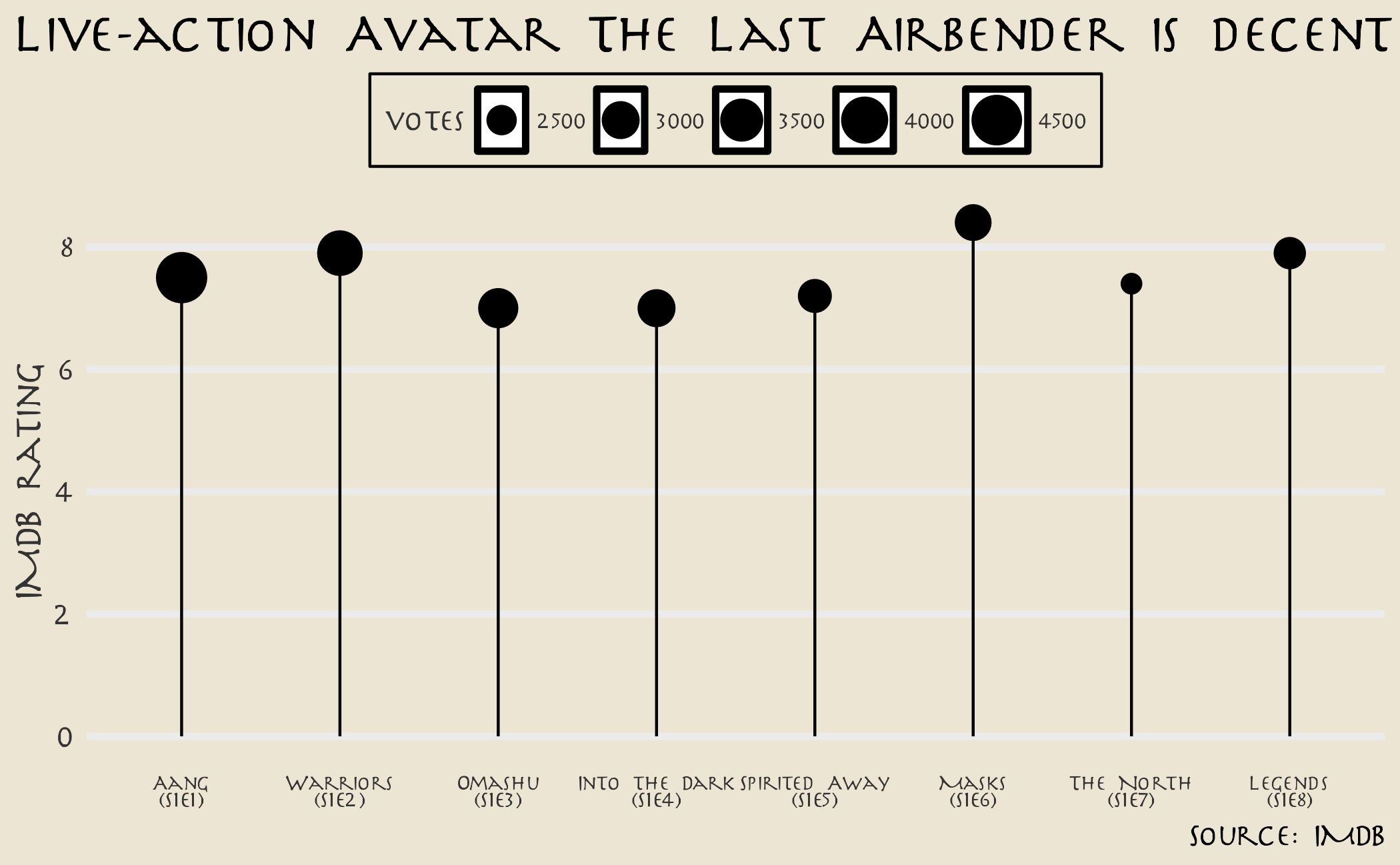
labs(
title = "Live-action Avatar The Last Airbender is decent",
x = NULL,
y = "IMDB rating",
caption = "Source: IMDB"
) +
# use an Avatar theme
theme_avatar(
# custom font
title.font = "Slayer",
text.font = "Slayer",
legend.font = "Slayer",
# shrink legend text size
legend.title.size = 8,
legend.text.size = 6
) +
theme(
# remove undesired grid lines
panel.grid.major.x = element_blank(),
panel.grid.minor.y = element_blank(),
# move legend to the top
legend.position = "top",
# align title flush with the edge
plot.title.position = "plot",
# shink x-axis text labels to fit
axis.text.x = element_text(size = rel(x = 0.7))
)