Models with transformations and multiple predictors

Lecture 17

Dr. Benjamin Soltoff

Cornell University
INFO 2950 - Spring 2024

March 21, 2024

Announcements

Announcements

• Project
  • Proposal feedback
  • EDA
• Homework 05

Goals

• Fit and interpret regression transformations
• Fit and interpret models with multiple predictors
• Distinguish between additive and interaction models

“Linear” models

“Linear” models

• We’re fitting a “linear” model, which assumes a linear relationship between our explanatory and response variables.
• But how do we assess this?

Assessing film quality

# A tibble: 146 × 5
   film                    audience critics genre     box_office
   <chr>                      <dbl>   <dbl> <chr>          <dbl>
 1 Avengers: Age of Ultron       86      74 Action     459005868
 2 Cinderella                    80      85 Adventure  201151353
 3 Ant-Man                       90      80 Action     180202163
 4 Do You Believe?               84      18 Drama       12985600
 5 Hot Tub Time Machine 2        28      14 Comedy      12314651
 6 The Water Diviner             62      63 Drama        4196641
 7 Irrational Man                53      42 Comedy       4030360
 8 Top Five                      64      86 Comedy      25317471
 9 Shaun the Sheep Movie         82      99 Animation   19375982
10 Love & Mercy                  87      89 Biography   12551031
# ℹ 136 more rows

Linear regression model

Graphical diagnostic: residual plot

• Plot
• Code
• Augment

aud_box_lm <- linear_reg() |>
  fit(audience ~ box_office, data = movie_scores)

aud_box_fit_aug <- augment(aud_box_lm$fit)

# plot the residuals
ggplot(
  data = aud_box_fit_aug,
  mapping = aes(x = .fitted, y = .resid)
) +
  geom_point(alpha = 0.5) +
  geom_hline(yintercept = 0, linetype = 2) +
  labs(
    x = "Fitted values",
    y = "Residuals"
  )

# A tibble: 141 × 9
   .rownames audience box_office .fitted  .resid    .hat .sigma    .cooksd
   <chr>        <dbl>      <dbl>   <dbl>   <dbl>   <dbl>  <dbl>      <dbl>
 1 1               86  459005868    77.7   8.27  0.135     19.9 0.0156    
 2 2               80  201151353    68.5  11.5   0.0237    19.9 0.00416   
 3 3               90  180202163    67.8  22.2   0.0193    19.8 0.0125    
 4 4               84   12985600    61.8  22.2   0.00852   19.8 0.00543   
 5 5               28   12314651    61.7 -33.7   0.00857   19.7 0.0126    
 6 6               62    4196641    61.5   0.544 0.00917   19.9 0.00000350
 7 7               53    4030360    61.5  -8.45  0.00918   19.9 0.000846  
 8 8               64   25317471    62.2   1.79  0.00781   19.9 0.0000321 
 9 9               82   19375982    62.0  20.0   0.00812   19.9 0.00418   
10 10              87   12551031    61.8  25.2   0.00855   19.8 0.00702   
# ℹ 131 more rows
# ℹ 1 more variable: .std.resid <dbl>

Looking for…

• Residuals distributed randomly around 0
• With no visible pattern along the x or y axes

Not looking for…

Fan shapes

Not looking for…

Groups of patterns

Not looking for…

Residuals correlated with predicted values

Not looking for…

Any patterns!

What patterns does the residuals plot reveal that should make us question whether a linear model is a good fit for modeling the relationship between audience scores and box office revenue?

Exploring linearity

Data: box office revenue

Box office vs. audience score

Which plot shows a more linear relationship?

Box office vs. audience score, residuals

Which plot shows residuals that are (more) uncorrelated with predicted values from the model? Also, what is the unit of the residuals?

Regression transformations

Transforming the data

• We saw that box_office has a right-skewed distribution, and the relationship between revenue and audience rating is non-linear.
• In these situations a transformation applied to the explanatory variable may be useful.
• In order to decide which transformation to use, we should examine the distribution of the explanatory variable.

What is a transformation?

• \(x \rightarrow f(x)\)

• Transformation functions are things like…
  • Squaring
  • Logarithms
  • Exponentiating
  • Adding/subtracting a constant

What is a transformation?

Can we use transformations with regressions?

• Original model

  \[\Large{Y = \beta_0 + \beta_1 X + \epsilon}\]

• Transformed model

  • \({\color{orange}f(Y)} = \beta_0 + \beta_1 X + \epsilon\)
  • \(Y = \beta_0 + \beta_1 {\color{orange}f(X)} + \epsilon\)
  • \({\color{orange}f(Y)} = \beta_0 + \beta_1 {\color{orange}f(X)} + \epsilon\)

• If \(f()\) is not linear (e.g. logarithmic, quadratic), are these still linear regressions?

Can we use transformations with regressions?

• Transformations (including non-linear ones) are used to achieve greater linearity in a linear regression model
• Transformations can allow for easier interpretability of your model and data

Which of these has a better linear fit?

When to use transformations with regressions

When the relationship between \(X\) and \(Y\) is non-linear.

1. Calculate your predicted errors \(\epsilon_i\) (residuals) from model \(\hat{Y} = b_0 + b_1 X\)
2. Plot the residuals on the \(y\)-axis against estimated \(\hat{y_i}\)s on the \(x\)-axis
   1. If they seem random, the data are \(\approx\) linear
   2. If not random, data are non-linear and need to be transformed

What does residual randomness have to do with linearity?

\[\Large{Y = {\color{orange}\beta_0 + \beta_1 X} + \color{blue}{\epsilon}}\]

• Deterministic (no randomness)
• Stochastic (random and unpredictable)

Why might residuals not be random?

The deterministic part of the model \(\color{orange}{\beta_0 + \beta_1 X}\) is not capturing all of the information hidden in your data, which is leaking into your residual

• Weird curvature – missing transformations
• Missing variables

Caution: Heteroskedasticity

• When the variance of the residuals are unequal
• This is a problem: linear regressions (OLS) assume constant variance for residuals
• We shouldn’t use OLS regressions if we don’t have constant variance

Caution: Heteroskedasticity

When does heteroskedasticity occur?

It depends on the data. Common examples include:

1. In time series – values changing in the same way over time
2. Massive range in values ($1 vs. $1,000,000)
3. Relationship between food expenditures and income

What to do when you have data with heteroskedasticity?

Use transforms

• Logarithm
• Square root
• Cube root

Logarithms smoosh big numbers

Which of these has a better linear fit?

Interpreting regressions with transformed variables

First derivative with respect to \(X\)

\[ \begin{aligned} \hat{Y} &= b_0 + b_1 X \\ \frac{\partial \hat{Y}}{\partial X} &= b_1 \end{aligned} \]

\[ \begin{aligned} \hat{Y} &= b_0 + b_1 X + b_2 X^2 \\ \frac{\partial \hat{Y}}{\partial X} &= b_1 + 2 b_2 X \end{aligned} \]

Difference in estimated value depends on starting value of \(X\)

Interpreting regressions with log-transformed variables

\[ \begin{aligned} \hat{Y} &= b_0 + b_1 X \\ \frac{\partial \hat{Y}}{\partial X} &= b_1 \end{aligned} \]

\[ \begin{aligned} \hat{Y} &= b_0 + b_1 \ln (X) \\ \frac{\partial \hat{Y}}{\partial X} &= b_1 \times \frac{1}{X} \\ &= \frac{b_1}{X} \end{aligned} \]

Interpreting regressions with natural logs

Model	Interpretation
\(\widehat{Y} = b_0 + b_1 X\)	For every one unit change in \(X\), we expect \(Y\) to be higher/lower by \(b_1\) units, on average.
\(\widehat{Y} = b_0 + b_1 \ln (X)\)	For every 1% change in \(X\), we expect \(Y\) to be higher/lower by \(0.01 \times b_1\) units, on average.
\(\widehat{\ln(Y)} = b_0 + b_1 X\)	For every one unit change in \(X\), we expect \(Y\) to be higher/lower by \(100 \times [\exp(b_1) - 1]\%\) units, on average.
\(\widehat{\ln(Y)} = b_0 + b_1 \ln (X)\)	For every 1% change in \(X\), we expect \(Y\) to be higher/lower by \(b_1\)%, on average.

Interpreting regressions with natural logs

# A tibble: 2 × 5
  term            estimate std.error statistic   p.value
  <chr>              <dbl>     <dbl>     <dbl>     <dbl>
1 (Intercept)       56.5      13.8       4.09  0.0000714
2 log(box_office)    0.418     0.835     0.500 0.618    

• Slope: For every 1% change in box office revenue, we expect the audience score to be higher by 0.004 points, on average.
• Intercept: Films with box office revenue of $1 (\(\ln(1) = 0\)) are expected to have an audience score of 56.45 points, on average.

Other common transformations

• Collapse numeric variables to discrete intervals
  • Reduce granularity
• Categorical data
  • \(X = \text{Cornell Campus}\) which takes only two values \(\{\text{Ithaca}, \text{Tech}\}\)
  • Instead map them to \(X = \text{Ithaca}\) where \(X = \{0, 1\}\)

Models with multiple predictors

Audience score vs. critics score and box office

• Audience score
• Critics score
• Box office revenue

audience	critics	box_office
86	74	$459M
80	85	$201M
90	80	$180M
84	18	$13M
28	14	$12M
62	63	$4M
...	...	...

Audience score vs. critics score and box office

linear_reg() |>
  fit(audience ~ critics, data = movie_scores) |>
  tidy()

# A tibble: 2 × 5
  term        estimate std.error statistic  p.value
  <chr>          <dbl>     <dbl>     <dbl>    <dbl>
1 (Intercept)   32.3      2.34        13.8 4.03e-28
2 critics        0.519    0.0345      15.0 2.70e-31

Audience score vs. critics score and box office

linear_reg() |>
  fit(audience ~ critics + log(box_office), data = movie_scores) |>
  tidy()

# A tibble: 3 × 5
  term            estimate std.error statistic  p.value
  <chr>              <dbl>     <dbl>     <dbl>    <dbl>
1 (Intercept)       -0.143    9.02     -0.0158 9.87e- 1
2 critics            0.544    0.0346   15.7    1.27e-32
3 log(box_office)    1.88     0.509     3.68   3.32e- 4

Interpretation of estimates

# A tibble: 3 × 5
  term            estimate std.error statistic  p.value
  <chr>              <dbl>     <dbl>     <dbl>    <dbl>
1 (Intercept)       -0.143    9.02     -0.0158 9.87e- 1
2 critics            0.544    0.0346   15.7    1.27e-32
3 log(box_office)    1.88     0.509     3.68   3.32e- 4

• Slope - audience: All else held constant, for every one point increase in the critics score, we expect the audience score to be higher by 0.54 points, on average.
• Slope - box office: All else held constant, for every 1% change in box office revenue, we expect the audience score to be higher by 0.019 points, on average.
• Intercept: Films with a critics score of 0 and no box office revenue are expected to have an audience score of -0.14 points, on average.

Interaction effects

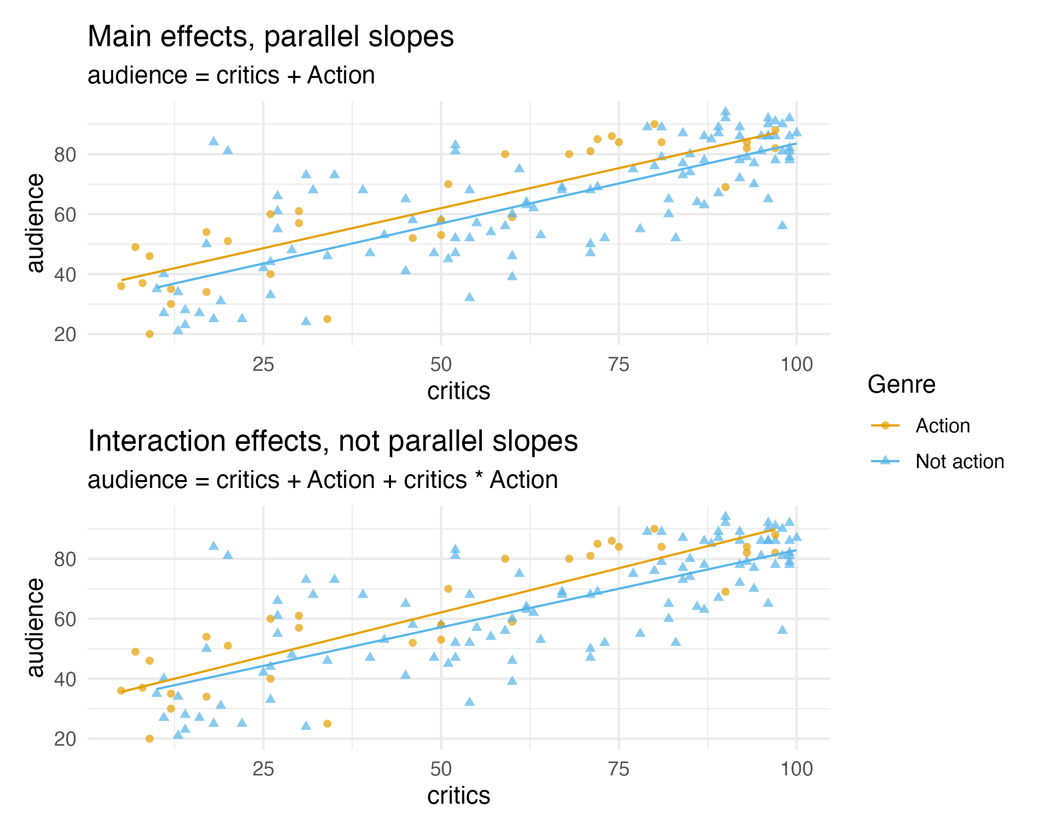
Main vs. interaction effects

Suppose we want to predict audience ratings based on critics’ ratings and whether or not it is an Action film. Do you think a model with main effects or interaction effects is more appropriate?

Hint: Main effects would mean the rate at which audience ratings change as critics’ ratings increase would be the same for Action and non-Action films, and interaction effects would mean the rate at which audience ratings change as critics’ ratings increase would be different for Action and non-Action films.

In pursuit of Occam’s razor

• Occam’s Razor states that among competing hypotheses that predict equally well, the one with the fewest assumptions should be selected.
• Model selection follows this principle.
• We only want to add another variable to the model if the addition of that variable brings something valuable in terms of predictive power to the model.
• In other words, we prefer the simplest best model, i.e. parsimonious model.

Visually, which of the two models is preferable under Occam’s razor?

R-squared

\[ R^2 = 1 - \frac{\text{variability in residuals}}{\text{variability in the outcome}} = 1 - \frac{\text{Var}(e_i)}{\text{Var}(y_i)} \]

where \(e_i\) represents the residuals of the model and \(y_i\) the outcomes.

\(R^2\) is the percentage of variability in the response variable explained by the regression model.

glance(ratings_main_fit)$r.squared

[1] 0.6167923

glance(ratings_int_fit)$r.squared

[1] 0.6190833

• Clearly the model with interactions has a higher \(R^2\).
• However using \(R^2\) for model selection in models with multiple explanatory variables is not a good idea as \(R^2\) increases when any variable is added to the model.

Adjusted R-squared

\[ \begin{aligned} R_{adj}^{2} &= 1 - \frac{s_{\text{residuals}}^2 / (n-k-1)} {s_{\text{outcome}}^2 / (n-1)} \\ &= 1 - \frac{s_{\text{residuals}}^2}{s_{\text{outcome}}^2} \times \frac{n-1}{n-k-1} \end{aligned} \]

where \(n\) is the number of observations used to fit the model and \(k\) is the number of predictor variables in the model.

• Adjusted \(R^2\) doesn’t increase if the new variable does not provide any new information or is completely unrelated, as it applies a penalty for number of variables included in the model.
• This makes adjusted \(R^2\) a preferable metric for model selection in multiple regression models.

Comparing models

glance(ratings_main_fit)$r.squared

[1] 0.6167923

glance(ratings_int_fit)$r.squared

[1] 0.6190833

glance(ratings_main_fit)$adj.r.squared

[1] 0.6113567

glance(ratings_int_fit)$adj.r.squared

[1] 0.6109208

• Is R-sq higher for int model?

glance(ratings_int_fit)$r.squared > glance(ratings_main_fit)$r.squared 

[1] TRUE

• Is R-sq adj. higher for int model?

glance(ratings_int_fit)$adj.r.squared > glance(ratings_main_fit)$adj.r.squared

[1] FALSE

Application exercise

ae-15

• Clone the repo in RStudio Workbench from this URL:

  https://github.com/info-2950/ae-15.git

• Open the Quarto document in the repo, and follow along and complete the exercises.

Recap of AE

• Linear regression assumes linearity between \(X\) and \(Y\). If this is not the case, you can use transformations to enforce linearity in the mapping between the two variables
• Multiple variable regression holds constant other explanations of the response variable
• Additive models assume the same slope between \(X\) and \(Y\), regardless of \(Z\). Interactive models allow for the slope to vary
• Use adjusted R-squared and other metrics to compare models
• Simpler models are preferable to complex models

Acknowledgments

• Draws upon material from Data Science in a Box licensed under Creative Commons Attribution-ShareAlike 4.0 International

Penguins