Models for discrete outcomes

Lecture 18

Dr. Benjamin Soltoff

Cornell University
INFO 2950 - Spring 2024

March 26, 2024

Announcements

Exam 01
Homework 05
Project EDA

Goals

Fit and interpret models for predicting binary outcomes
Evaluate the performance of these models
Determine appropriate decision thresholds
Implement train/test set splits for model validation

Predicting categorical data

Spam filters

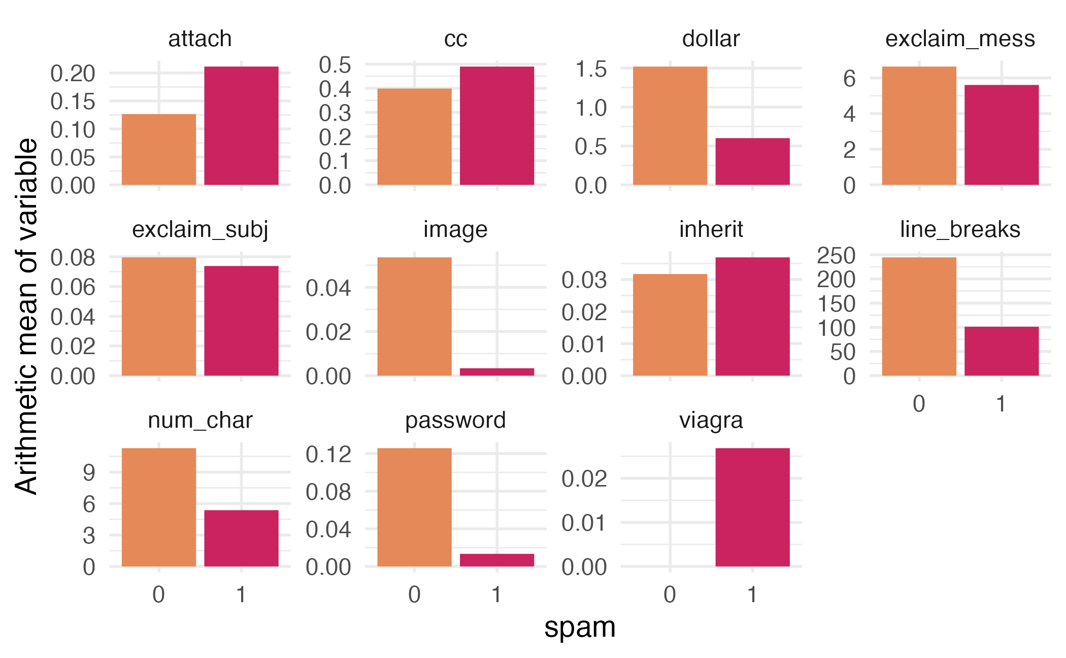
Data from 3921 emails and 21 variables on them
Outcome: whether the email is spam or not
Predictors:
- Number of characters
- Whether the email had “Re:” in the subject
- Number of times the word “inherit” shows up in the email
- Etc.

library(openintro)
glimpse(email)

Rows: 3,921
Columns: 21
$ spam         <fct> 0, 0, 0, 0, 0, 0, 0, 0, 0, 0, 0, 0, 0…
$ to_multiple  <fct> 0, 0, 0, 0, 0, 0, 1, 1, 0, 0, 0, 0, 0…
$ from         <fct> 1, 1, 1, 1, 1, 1, 1, 1, 1, 1, 1, 1, 1…
$ cc           <int> 0, 0, 0, 0, 0, 0, 0, 1, 0, 0, 0, 1, 0…
$ sent_email   <fct> 0, 0, 0, 0, 0, 0, 1, 1, 0, 0, 1, 0, 0…
$ time         <dttm> 2012-01-01 01:16:41, 2012-01-01 02:0…
$ image        <dbl> 0, 0, 0, 0, 0, 0, 0, 1, 0, 0, 0, 0, 0…
$ attach       <dbl> 0, 0, 0, 0, 0, 0, 0, 1, 0, 0, 0, 0, 0…
$ dollar       <dbl> 0, 0, 4, 0, 0, 0, 0, 0, 0, 0, 0, 0, 0…
$ winner       <fct> no, no, no, no, no, no, no, no, no, n…
$ inherit      <dbl> 0, 0, 1, 0, 0, 0, 0, 0, 0, 0, 0, 0, 0…
$ viagra       <dbl> 0, 0, 0, 0, 0, 0, 0, 0, 0, 0, 0, 0, 0…
$ password     <dbl> 0, 0, 0, 0, 2, 2, 0, 0, 0, 0, 0, 0, 0…
$ num_char     <dbl> 11.370, 10.504, 7.773, 13.256, 1.231,…
$ line_breaks  <int> 202, 202, 192, 255, 29, 25, 193, 237,…
$ format       <fct> 1, 1, 1, 1, 0, 0, 1, 1, 0, 1, 1, 0, 1…
$ re_subj      <fct> 0, 0, 0, 0, 0, 0, 0, 0, 0, 0, 0, 1, 0…
$ exclaim_subj <dbl> 0, 0, 0, 0, 0, 0, 0, 0, 0, 0, 0, 0, 0…
$ urgent_subj  <fct> 0, 0, 0, 0, 0, 0, 0, 0, 0, 0, 0, 0, 0…
$ exclaim_mess <dbl> 0, 1, 6, 48, 1, 1, 1, 18, 1, 0, 2, 1,…
$ number       <fct> big, small, small, small, none, none,…

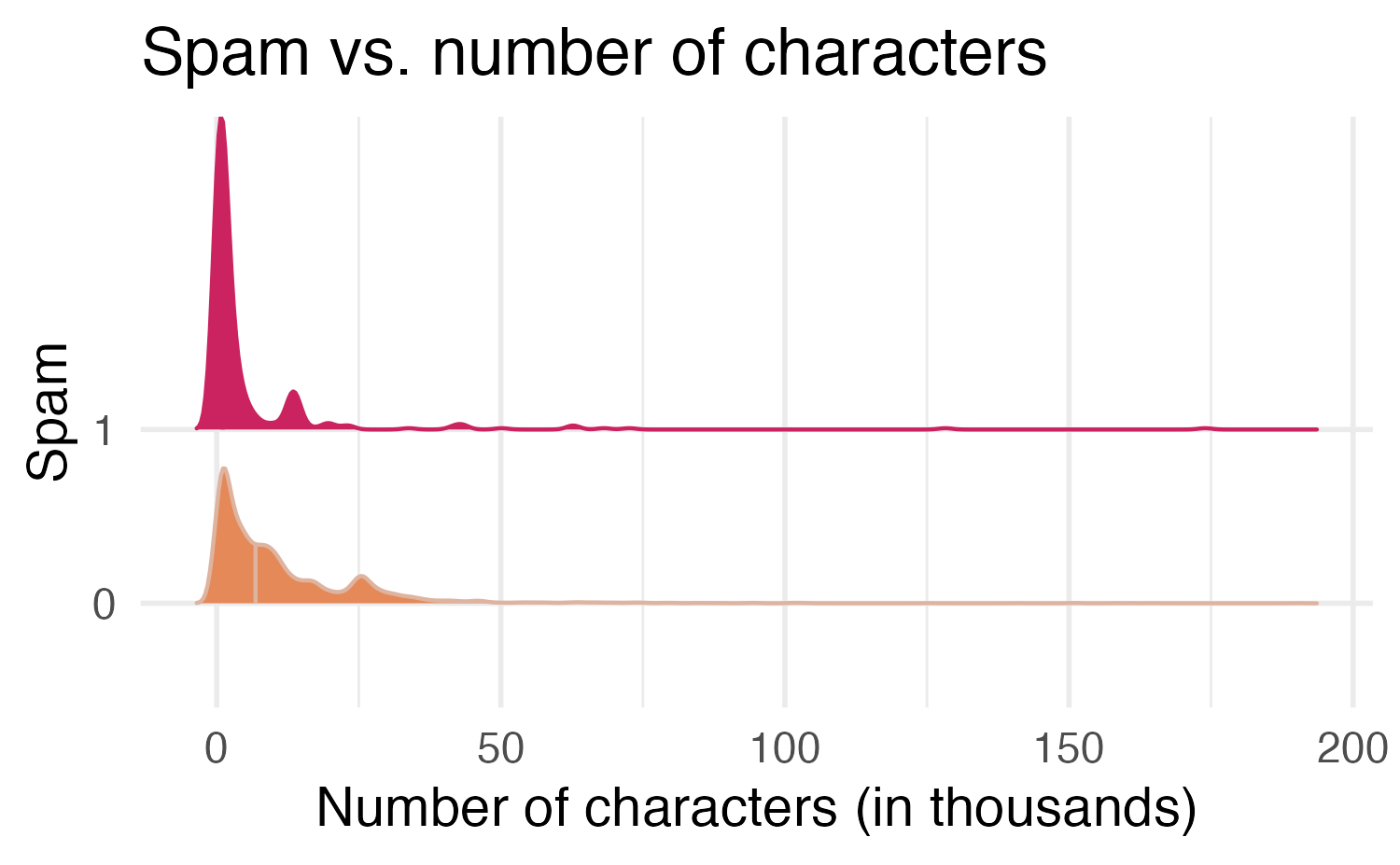
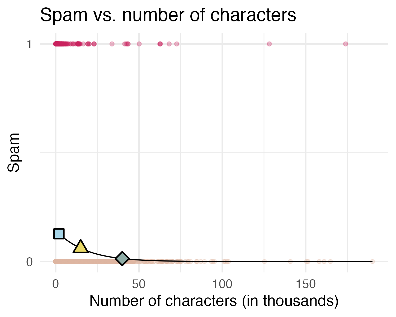
Would you expect longer or shorter emails to be spam?

# A tibble: 2 × 2
  spam  mean_num_char
  <fct>         <dbl>
1 0             11.3 
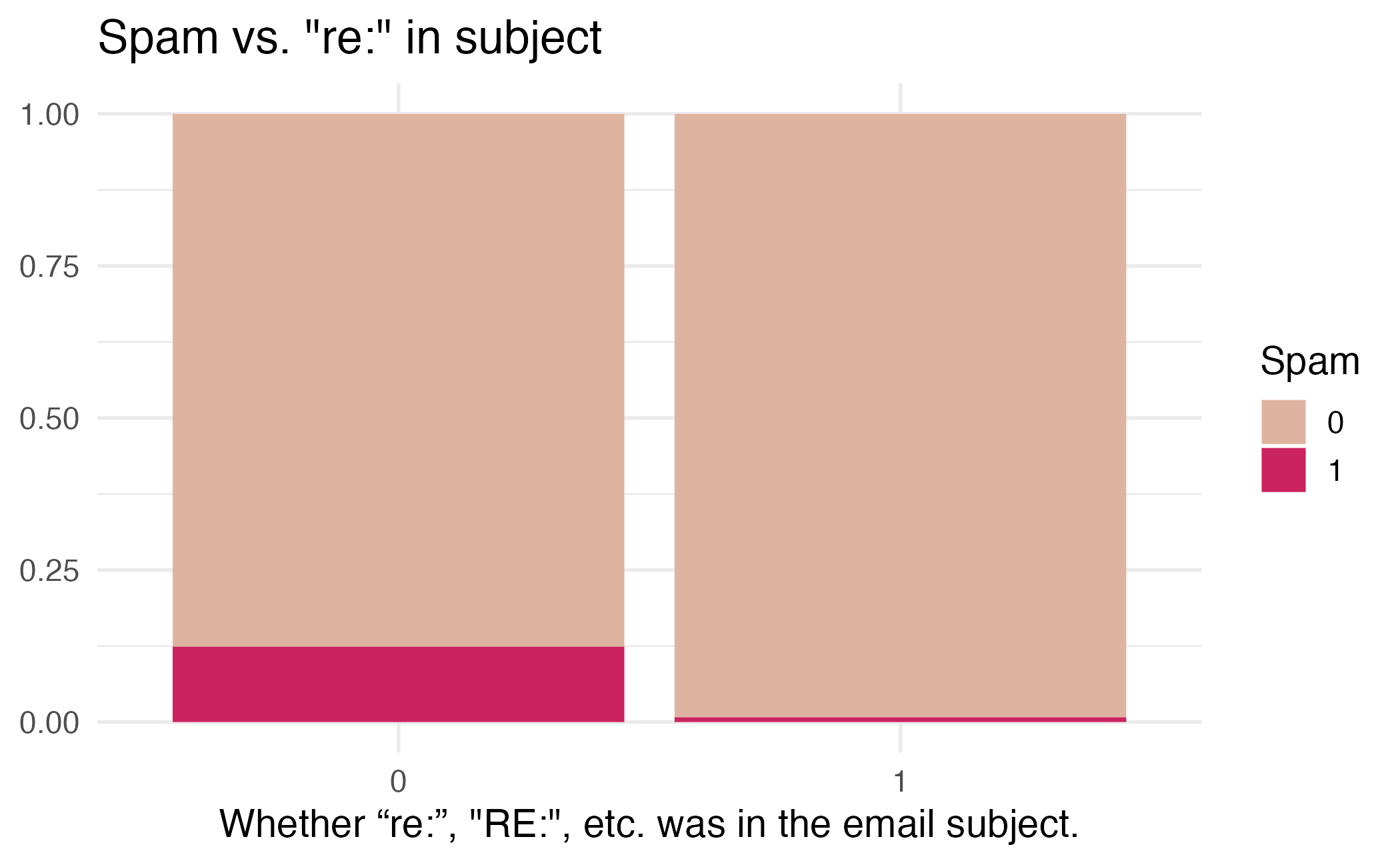
2 1              5.44

Would you expect emails that have subjects starting with “Re:”, “RE:”, “re:”, or “rE:” to be spam or not?

Modelling spam

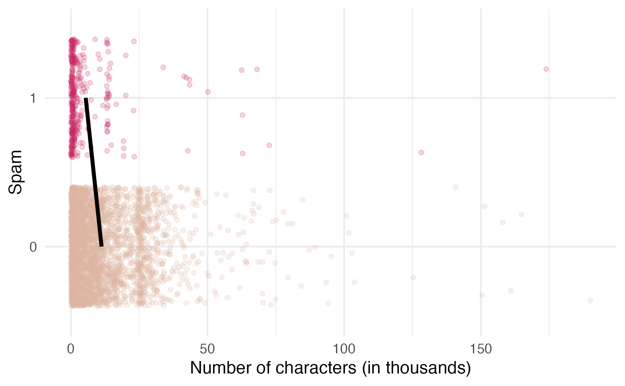
Both number of characters and whether the message has “re:” in the subject might be related to whether the email is spam. How do we come up with a model that will let us explore this relationship?
For simplicity, we’ll focus on the number of characters (num_char) as predictor, but the model we describe can be expanded to take multiple predictors as well.

Modelling spam

This isn’t something we can reasonably fit a linear model to – we need something different!

Feel the Bern(oulli)

Framing the problem

We can treat each outcome (spam and not) as successes and failures arising from separate Bernoulli trials
- Bernoulli trial: a random experiment with exactly two possible outcomes, “success” and “failure”, in which the probability of success is the same every time the experiment is conducted
Each Bernoulli trial can have a separate probability of success

\[ y_i ∼ \text{Bern}(p_i)\]
We can then use the predictor variables to model that probability of success, \(p_i\)
We can’t just use a linear model for \(p_i\) (since \(p_i\) must be between 0 and 1) but we can transform the linear model to have the appropriate range

Generalized linear models

This is a very general way of addressing many problems in regression and the resulting models are called generalized linear models (GLMs)
Logistic regression is just one example
- Binary outcomes
- Ordinal outcomes
- Nominal outcomes
- Event counts
- Survival/duration models
- Continuous outcomes

Three characteristics of GLMs

A probability distribution describing a data generating process for the outcome variable
A linear model: \[\eta = \beta_0 + \beta_1 X_1 + \cdots + \beta_k X_k\]
A link function that relates the linear model to the parameter of the outcome distribution

Logistic regression

Logistic regression is a GLM used to model a binary categorical outcome using numerical and categorical predictors
To finish specifying the logistic model we need to define a reasonable link function that connects \(\eta_i\) to \(p_i\): logit function
Logit function: For \(0\le p \le 1\)

\[\text{logit}(p) = \log\left(\frac{p}{1-p}\right)\]

Logit function, visualized

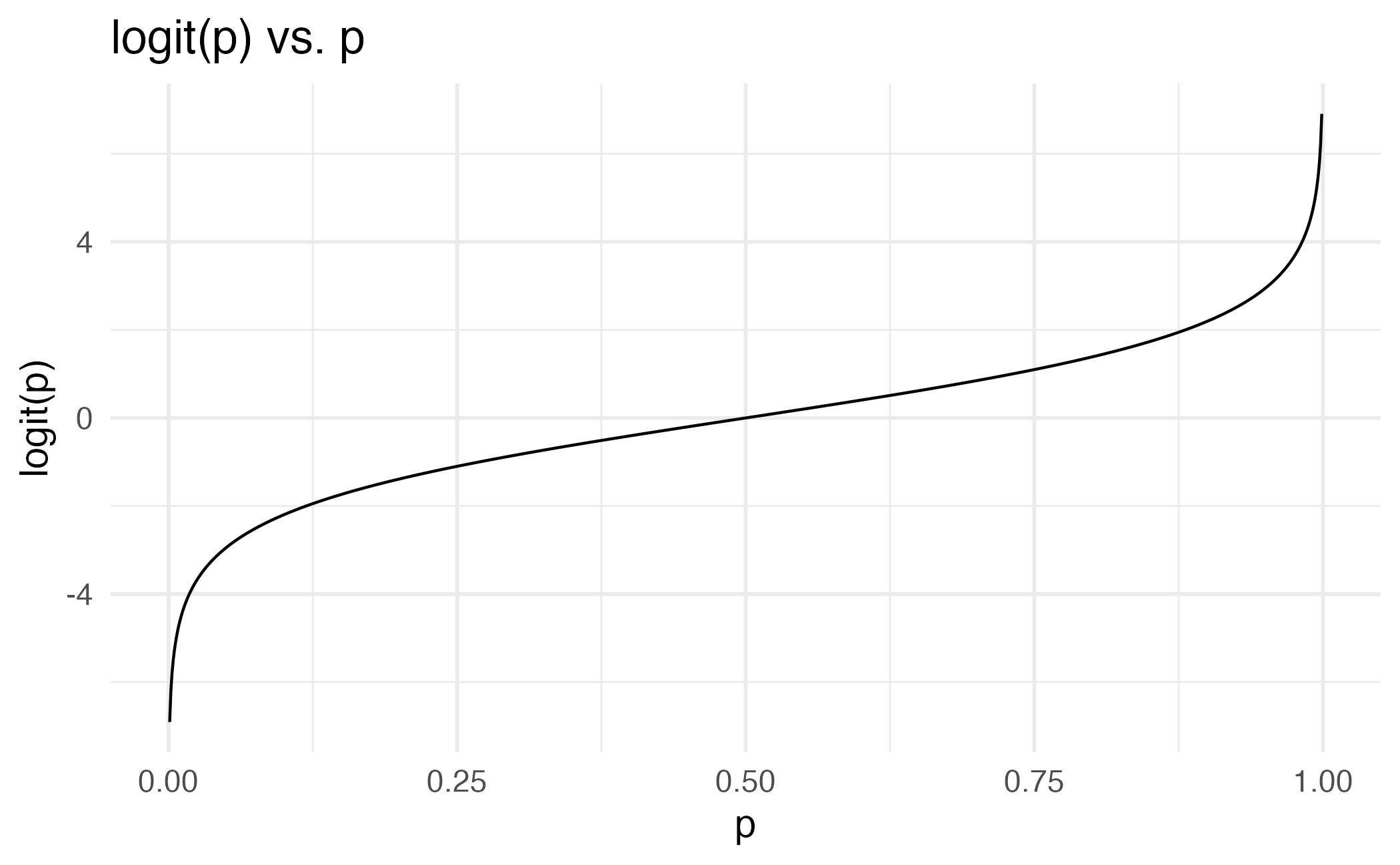
Properties of the logit

The logit function takes a value between 0 and 1 and maps it to a value between \(-\infty\) and \(\infty\)
Inverse logit (logistic) function:

\[g^{-1}(x) = \frac{\exp(x)}{1+\exp(x)} = \frac{1}{1+\exp(-x)}\]
The inverse logit function takes a value between \(-\infty\) and \(\infty\) and maps it to a value between 0 and 1

The logistic regression model

Based on the three GLM criteria we have
- \(y_i \sim \text{Bern}(p_i)\)
- \(\eta_i = \beta_0+\beta_1 x_{1,i} + \cdots + \beta_n x_{n,i}\)
- \(\text{logit}(p_i) = \eta_i\)
From which we get

\[p_i = \frac{\exp(\beta_0+\beta_1 x_{1,i} + \cdots + \beta_k x_{k,i})}{1+\exp(\beta_0+\beta_1 x_{1,i} + \cdots + \beta_k x_{k,i})}\]

Modeling spam

In R we fit a GLM in the same way as a linear model except we specify the model with logistic_reg()

spam_fit <- logistic_reg() |>
  fit(spam ~ num_char, data = email)

tidy(spam_fit)

# A tibble: 2 × 5
  term        estimate std.error statistic   p.value
  <chr>          <dbl>     <dbl>     <dbl>     <dbl>
1 (Intercept)  -1.80     0.0716     -25.1  2.04e-139
2 num_char     -0.0621   0.00801     -7.75 9.50e- 15

Spam model

tidy(spam_fit)

# A tibble: 2 × 5
  term        estimate std.error statistic   p.value
  <chr>          <dbl>     <dbl>     <dbl>     <dbl>
1 (Intercept)  -1.80     0.0716     -25.1  2.04e-139
2 num_char     -0.0621   0.00801     -7.75 9.50e- 15

Model:

\[\log\left(\frac{p}{1-p}\right) = -1.80 -0.06 \times \text{num\_char}\]

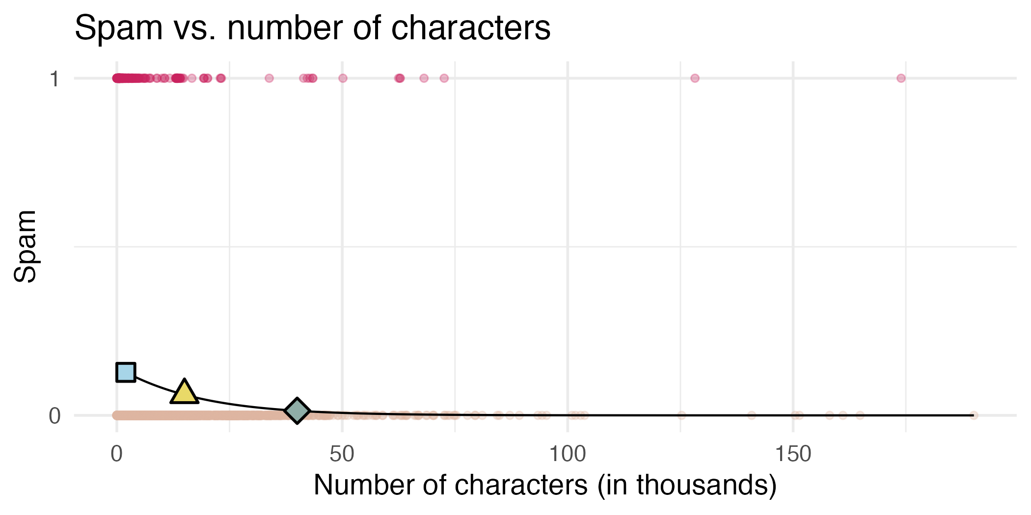
\(\Pr(\text{spam})\) for an email with 2000 characters

\[\log\left(\frac{p}{1-p}\right) = -1.80-0.0621\times 2 = -1.9242\]

\[\frac{p}{1-p} = \exp(-1.9242) = 0.15 \rightarrow p = 0.15 \times (1 - p)\]

\[p = 0.15 - 0.15p \rightarrow 1.15p = 0.15\]

\[p = 0.15 / 1.15 = 0.13\]

What is the probability that an email with 15,000 characters is spam? What about an email with 40,000 characters?

2K chars: \(\Pr(\text{spam}) = 0.13\)
15K chars: \(\Pr(\text{spam}) = 0.06\)
40K chars: \(\Pr(\text{spam}) = 0.01\)

Would you prefer an email with 2000 characters to be labelled as spam or not? How about 40,000 characters?

Sensitivity and specificity

False positive and negative

	Email is spam	Email is not spam
Email labelled spam	True positive	False positive (Type 1 error)
Email labelled not spam	False negative (Type 2 error)	True negative

False negative rate = Pr(Labelled not spam | Email spam) = FN / (TP + FN)
False positive rate = Pr(Labelled spam | Email not spam) = FP / (FP + TN)

Sensitivity and specificity

	Email is spam	Email is not spam
Email labelled spam	True positive	False positive (Type 1 error)
Email labelled not spam	False negative (Type 2 error)	True negative

Sensitivity = Pr(Labelled spam | Email spam) = TP / (TP + FN)
- Sensitivity = 1 − False negative rate
- Probability that the model identifies spam given that the email is spam

Specificity = Pr(Labelled not spam | Email not spam) = TN / (FP + TN)
- Specificity = 1 − False positive rate
- Probability that the model identifies not spam given that the email is not spam

If you were designing a spam filter, would you want sensitivity and specificity to be high or low? What are the trade-offs associated with each decision?

Prediction

Goal: Building a spam filter

Data: Set of emails and we know if each email is spam/not and other features
Use logistic regression to predict the probability that an incoming email is spam
Use model selection to pick the model with the best predictive performance

Building a model to predict the probability that an email is spam is only half of the battle! We also need a decision rule about which emails get flagged as spam (e.g. what probability should we use as out cutoff?)

A simple approach: choose a single threshold probability and any email that exceeds that probability is flagged as spam

# A tibble: 22 × 5
   term         estimate std.error statistic  p.value
   <chr>           <dbl>     <dbl>     <dbl>    <dbl>
 1 (Intercept)  -9.09e+1   9.80e+3  -0.00928 9.93e- 1
 2 to_multiple1 -2.68e+0   3.27e-1  -8.21    2.25e-16
 3 from1        -2.19e+1   9.80e+3  -0.00224 9.98e- 1
 4 cc            1.88e-2   2.20e-2   0.855   3.93e- 1
 5 sent_email1  -2.07e+1   3.87e+2  -0.0536  9.57e- 1
 6 time          8.48e-8   2.85e-8   2.98    2.92e- 3
 7 image        -1.78e+0   5.95e-1  -3.00    2.73e- 3
 8 attach        7.35e-1   1.44e-1   5.09    3.61e- 7
 9 dollar       -6.85e-2   2.64e-2  -2.59    9.64e- 3
10 winneryes     2.07e+0   3.65e-1   5.67    1.41e- 8
11 inherit       3.15e-1   1.56e-1   2.02    4.32e- 2
12 viagra        2.84e+0   2.22e+3   0.00128 9.99e- 1
13 password     -8.54e-1   2.97e-1  -2.88    4.03e- 3
14 num_char      5.06e-2   2.38e-2   2.13    3.35e- 2
15 line_breaks  -5.49e-3   1.35e-3  -4.06    4.91e- 5
16 format1      -6.14e-1   1.49e-1  -4.14    3.53e- 5
17 re_subj1     -1.64e+0   3.86e-1  -4.25    2.16e- 5
18 exclaim_subj  1.42e-1   2.43e-1   0.585   5.58e- 1
19 urgent_subj1  3.88e+0   1.32e+0   2.95    3.18e- 3
20 exclaim_mess  1.08e-2   1.81e-3   5.98    2.23e- 9
21 numbersmall  -1.19e+0   1.54e-1  -7.74    9.62e-15
22 numberbig    -2.95e-1   2.20e-1  -1.34    1.79e- 1

logistic_reg() |>
  fit(spam ~ ., data = email) |>
  tidy() |>
  print(n = 22)

Prediction

The mechanics of prediction is easy:
- Plug in values of predictors to the model equation
- Calculate the predicted value of the response variable, \(\hat{y}\)
Getting it right is hard!
- There is no guarantee the model estimates you have are correct
- Or that your model will perform as well with new data as it did with your sample data

Underfitting and overfitting

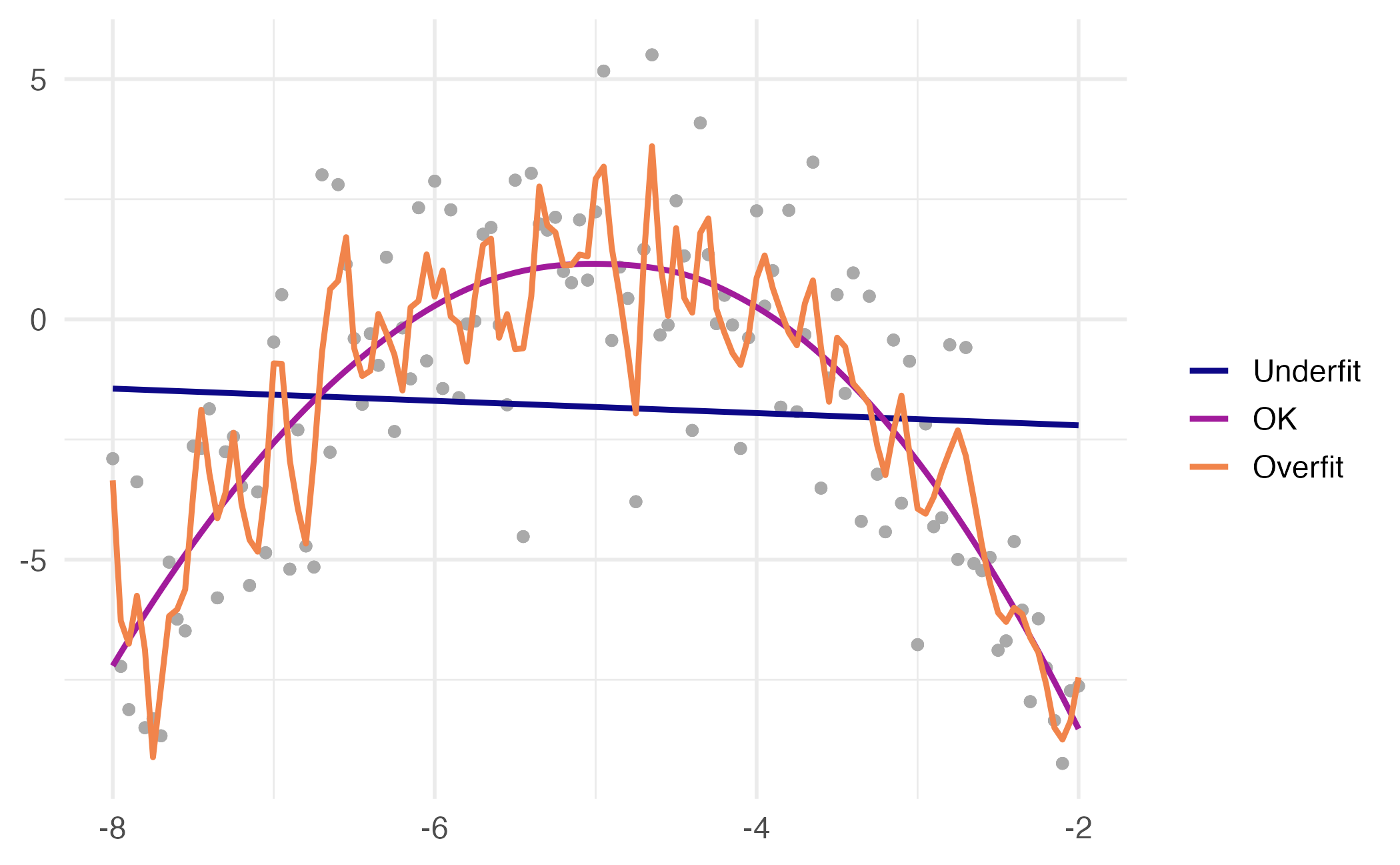
Spending our data

Several steps to create a useful model: parameter estimation, model selection, performance assessment, etc.
Doing all of this on the entire data we have available can lead to overfitting
Allocate specific subsets of data for different tasks, as opposed to allocating the largest possible amount to the model parameter estimation only (which is what we’ve done so far)

Splitting data

Training set:
- Sandbox for model building
- Spend most of your time using the training set to develop the model
- Majority of the data (usually 80%)
Testing set:
- Held in reserve to determine efficacy of one or two chosen models
- Critical to look at it once, otherwise it becomes part of the modeling process
- Remainder of the data (usually 20%)

Performing the split

# Fix random numbers by setting the seed 
# Enables analysis to be reproducible when random numbers are used 
set.seed(123)

# Put 80% of the data into the training set 
email_split <- initial_split(email, prop = 0.80)

# Create data frames for the two sets:
train_data <- training(email_split)
test_data  <- testing(email_split)

Peek at the split

glimpse(train_data)

Rows: 3,136
Columns: 21
$ spam         <fct> 0, 1, 0, 0, 0, 0, 0, 0…
$ to_multiple  <fct> 0, 0, 0, 1, 0, 0, 0, 0…
$ from         <fct> 1, 1, 1, 1, 1, 1, 1, 1…
$ cc           <int> 0, 0, 6, 0, 0, 0, 0, 0…
$ sent_email   <fct> 0, 0, 1, 0, 1, 0, 0, 1…
$ time         <dttm> 2012-02-29 15:19:00, …
$ image        <dbl> 0, 0, 1, 0, 0, 0, 0, 0…
$ attach       <dbl> 0, 0, 1, 1, 0, 0, 0, 0…
$ dollar       <dbl> 0, 0, 0, 2, 0, 1, 0, 0…
$ winner       <fct> no, no, no, no, no, no…
$ inherit      <dbl> 0, 0, 0, 0, 0, 0, 0, 0…
$ viagra       <dbl> 0, 0, 0, 0, 0, 0, 0, 0…
$ password     <dbl> 0, 0, 0, 0, 0, 0, 0, 0…
$ num_char     <dbl> 7.979, 0.496, 30.279, …
$ line_breaks  <int> 174, 13, 983, 37, 49, …
$ format       <fct> 1, 1, 1, 0, 1, 1, 1, 1…
$ re_subj      <fct> 0, 0, 1, 0, 1, 0, 0, 1…
$ exclaim_subj <dbl> 1, 0, 0, 0, 0, 0, 0, 0…
$ urgent_subj  <fct> 0, 0, 0, 0, 0, 0, 0, 0…
$ exclaim_mess <dbl> 8, 0, 31, 4, 2, 0, 2, …
$ number       <fct> small, none, big, smal…

glimpse(test_data)

Rows: 785
Columns: 21
$ spam         <fct> 0, 0, 0, 0, 0, 0, 0, 0…
$ to_multiple  <fct> 0, 0, 0, 0, 1, 1, 0, 0…
$ from         <fct> 1, 1, 1, 1, 1, 1, 1, 1…
$ cc           <int> 0, 0, 1, 0, 1, 2, 0, 0…
$ sent_email   <fct> 0, 0, 1, 0, 0, 0, 0, 0…
$ time         <dttm> 2012-01-01 11:00:32, …
$ image        <dbl> 0, 0, 0, 2, 0, 0, 0, 0…
$ attach       <dbl> 0, 0, 0, 2, 0, 0, 0, 0…
$ dollar       <dbl> 4, 0, 0, 9, 0, 0, 0, 1…
$ winner       <fct> no, no, no, no, no, no…
$ inherit      <dbl> 1, 0, 0, 0, 1, 0, 0, 0…
$ viagra       <dbl> 0, 0, 0, 0, 0, 0, 0, 0…
$ password     <dbl> 0, 2, 0, 0, 0, 0, 0, 0…
$ num_char     <dbl> 7.773, 1.091, 15.075, …
$ line_breaks  <int> 192, 25, 354, 344, 558…
$ format       <fct> 1, 0, 1, 1, 1, 0, 1, 1…
$ re_subj      <fct> 0, 0, 1, 0, 1, 1, 0, 0…
$ exclaim_subj <dbl> 0, 0, 0, 0, 0, 0, 0, 1…
$ urgent_subj  <fct> 0, 0, 0, 0, 0, 0, 0, 0…
$ exclaim_mess <dbl> 6, 1, 10, 4, 6, 3, 0, …
$ number       <fct> small, none, small, bi…

Modeling workflow

Fit a model to the training dataset

email_fit <- logistic_reg() |>
  fit(spam ~ ., data = train_data)

Categorical predictors

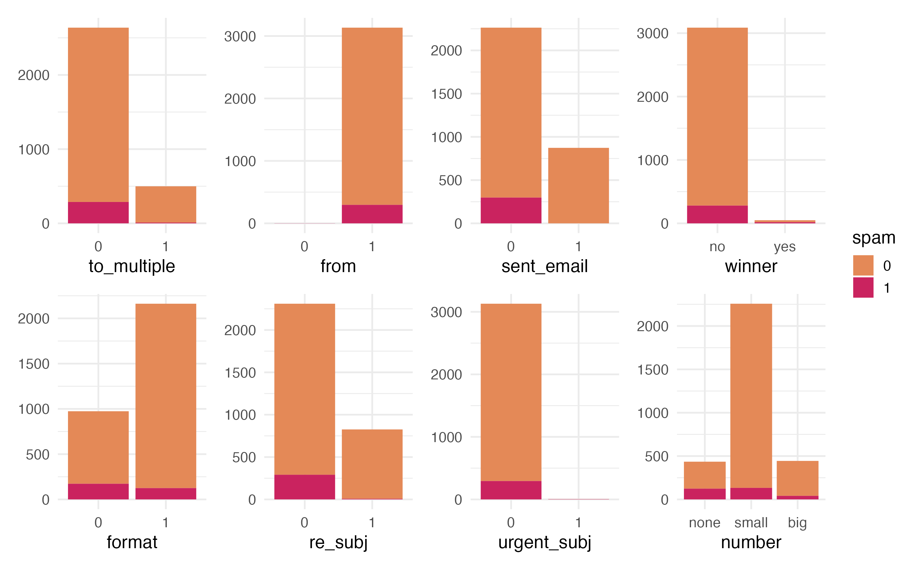
`from` and `sent_email`

from: Whether the message was listed as from anyone (this is usually set by default for regular outgoing email)

train_data |>
  count(spam, from)

# A tibble: 3 × 3
  spam  from      n
  <fct> <fct> <int>
1 0     1      2838
2 1     0         2
3 1     1       296

sent_email: Indicator for whether the sender had been sent an email in the last 30 days

train_data |>
  count(spam, sent_email)

# A tibble: 3 × 3
  spam  sent_email     n
  <fct> <fct>      <int>
1 0     0           1965
2 0     1            873
3 1     0            298

Numerical predictors

Fit a model to the training dataset

email_fit <- logistic_reg() |>
  fit(spam ~ . - from - sent_email - viagra, data = train_data)

email_fit

parsnip model object


Call:  stats::glm(formula = spam ~ . - from - sent_email - viagra, family = stats::binomial, 
    data = data)

Coefficients:
 (Intercept)  to_multiple1            cc          time         image  
  -7.558e+01    -2.701e+00     4.864e-02     5.655e-08    -3.165e+00  
      attach        dollar     winneryes       inherit      password  
   5.441e-01    -8.712e-02     2.484e+00     3.130e-01    -1.015e+00  
    num_char   line_breaks       format1      re_subj1  exclaim_subj  
   8.545e-02    -6.636e-03    -8.370e-01    -3.016e+00     4.813e-02  
urgent_subj1  exclaim_mess   numbersmall     numberbig  
   4.726e+00     9.492e-03    -8.511e-01     6.731e-03  

Degrees of Freedom: 3135 Total (i.e. Null);  3117 Residual
Null Deviance:      1969 
Residual Deviance: 1423     AIC: 1461

Predict outcome on the testing dataset

predict(email_fit, new_data = test_data)

# A tibble: 785 × 1
   .pred_class
   <fct>      
 1 0          
 2 0          
 3 0          
 4 0          
 5 0          
 6 0          
 7 0          
 8 0          
 9 0          
10 0          
# ℹ 775 more rows

Predict probabilities on the testing dataset

email_pred <- predict(email_fit, new_data = test_data, type = "prob") |>
  bind_cols(test_data |> select(spam, time))

email_pred

# A tibble: 785 × 4
   .pred_0  .pred_1 spam  time               
     <dbl>    <dbl> <fct> <dttm>             
 1   0.948 0.0522   0     2012-01-01 11:00:32
 2   0.938 0.0620   0     2012-01-01 05:04:46
 3   0.998 0.00194  0     2012-01-01 14:38:32
 4   1.00  0.000160 0     2012-01-01 21:05:47
 5   0.999 0.000505 0     2012-01-02 10:27:07
 6   0.999 0.000531 0     2012-01-02 16:24:21
 7   0.954 0.0459   0     2012-01-02 20:07:17
 8   0.985 0.0149   0     2012-01-03 04:34:50
 9   0.898 0.102    0     2012-01-03 09:20:23
10   0.681 0.319    0     2012-01-03 04:29:15
# ℹ 775 more rows

A closer look at predictions

email_pred |>
  arrange(desc(.pred_1)) |>
  print(n = 10)

# A tibble: 785 × 4
   .pred_0 .pred_1 spam  time               
     <dbl>   <dbl> <fct> <dttm>             
 1   0.188   0.812 0     2012-02-08 13:34:24
 2   0.300   0.700 1     2012-02-29 02:55:56
 3   0.312   0.688 1     2012-03-28 02:09:28
 4   0.335   0.665 0     2012-01-17 11:05:51
 5   0.351   0.649 0     2012-01-14 04:03:03
 6   0.358   0.642 1     2012-02-14 14:45:19
 7   0.363   0.637 1     2012-01-04 10:36:23
 8   0.379   0.621 1     2012-01-25 11:17:54
 9   0.395   0.605 0     2012-01-13 23:47:58
10   0.409   0.591 0     2012-01-31 10:07:48
# ℹ 775 more rows

Evaluate the performance

Receiver operating characteristic (ROC) curve¹ which plot true positive rate (sensitivity) vs. false positive rate (1 - specificity) across varying prediction thresholds

email_pred |>
  roc_curve(
    truth = spam,
    .pred_1,
    event_level = "second"
  ) |>
  autoplot()

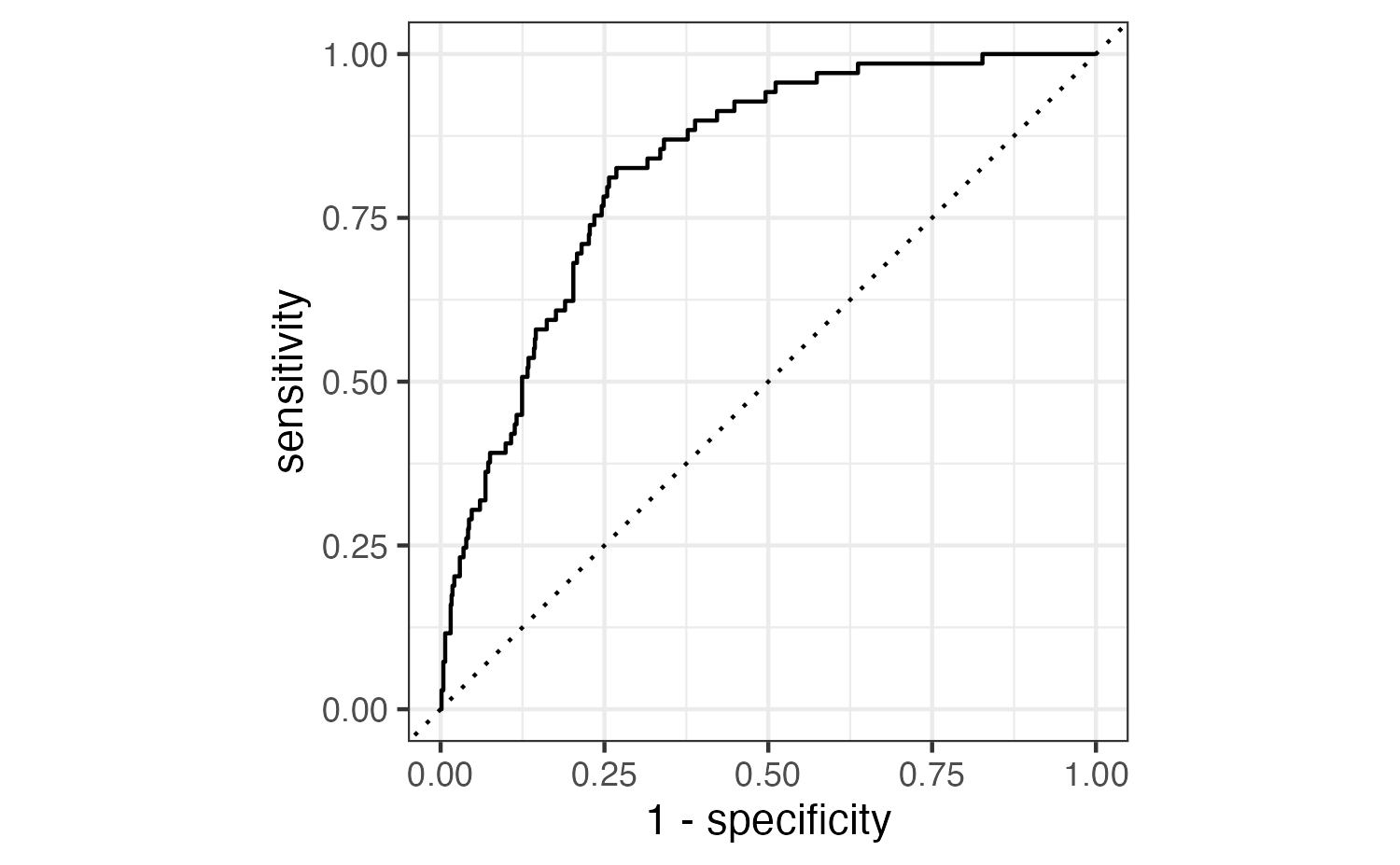
Evaluate the performance

Find the area under the curve:

email_pred |>
  roc_auc(
    truth = spam,
    .pred_1,
    event_level = "second"
  )

# A tibble: 1 × 3
  .metric .estimator .estimate
  <chr>   <chr>          <dbl>
1 roc_auc binary         0.828

Application exercise

Art history

Rows: 2,325
Columns: 24
$ artist_name            <chr> "Aaron Douglas", "Aaron Douglas", "Aaron Dougla…
$ edition_number         <dbl> 9, 10, 11, 12, 13, 14, 15, 16, 14, 15, 16, 5, 6…
$ title_of_work          <chr> "Noah's Ark", "Noah's Ark", "Noah's Ark", "Noah…
$ publication_year       <dbl> 1991, 1996, 2001, 2005, 2009, 2013, 2016, 2020,…
$ page_number_of_image   <chr> "965", "1053", "1030", "990", "937", "867", "91…
$ artist_unique_id       <dbl> 1, 1, 1, 1, 1, 1, 1, 1, 2, 2, 2, 3, 3, 3, 3, 3,…
$ artist_nationality     <chr> "American", "American", "American", "American",…
$ artist_gender          <chr> "Male", "Male", "Male", "Male", "Male", "Male",…
$ artist_race            <chr> "Black or African American", "Black or African …
$ artist_ethnicity       <chr> "Not Hispanic or Latinx", "Not Hispanic or Lati…
$ height_of_work_in_book <dbl> 11.3, 12.1, 12.3, 12.3, 12.8, 12.8, 12.7, 7.9, …
$ width_of_work_in_book  <dbl> 8.5, 8.9, 8.8, 8.8, 9.3, 9.3, 9.2, 19.0, 10.2, …
$ height_of_text         <dbl> 14.5, 12.4, 10.8, 15.7, 15.0, 18.8, 21.2, 14.7,…
$ width_of_text          <dbl> 8.4, 9.0, 9.0, 8.9, 9.3, 9.3, 9.2, 13.9, 9.3, 9…
$ extra_text_height      <dbl> 0.0, 0.0, 0.0, 0.0, 0.0, 0.0, 0.0, 0.0, 9.2, 0.…
$ extra_text_width       <dbl> 0.0, 0.0, 0.0, 0.0, 0.0, 0.0, 0.0, 0.0, 8.8, 0.…
$ area_of_work_in_book   <dbl> 96.05, 107.69, 108.24, 108.24, 119.04, 119.04, …
$ area_of_text           <dbl> 121.80, 111.60, 97.20, 139.73, 139.50, 174.84, …
$ extra_text_area        <dbl> 0.00, 0.00, 0.00, 0.00, 0.00, 0.00, 0.00, 0.00,…
$ total_area_text        <dbl> 121.80, 111.60, 97.20, 139.73, 139.50, 174.84, …
$ total_space            <dbl> 217.85, 219.29, 205.44, 247.97, 258.54, 293.88,…
$ page_area              <dbl> 616.500, 586.420, 677.440, 657.660, 648.930, 64…
$ space_ratio_per_page   <dbl> 0.3533658, 0.3739470, 0.3032593, 0.3770489, 0.3…
$ book                   <chr> "gardner", "gardner", "gardner", "gardner", "ga…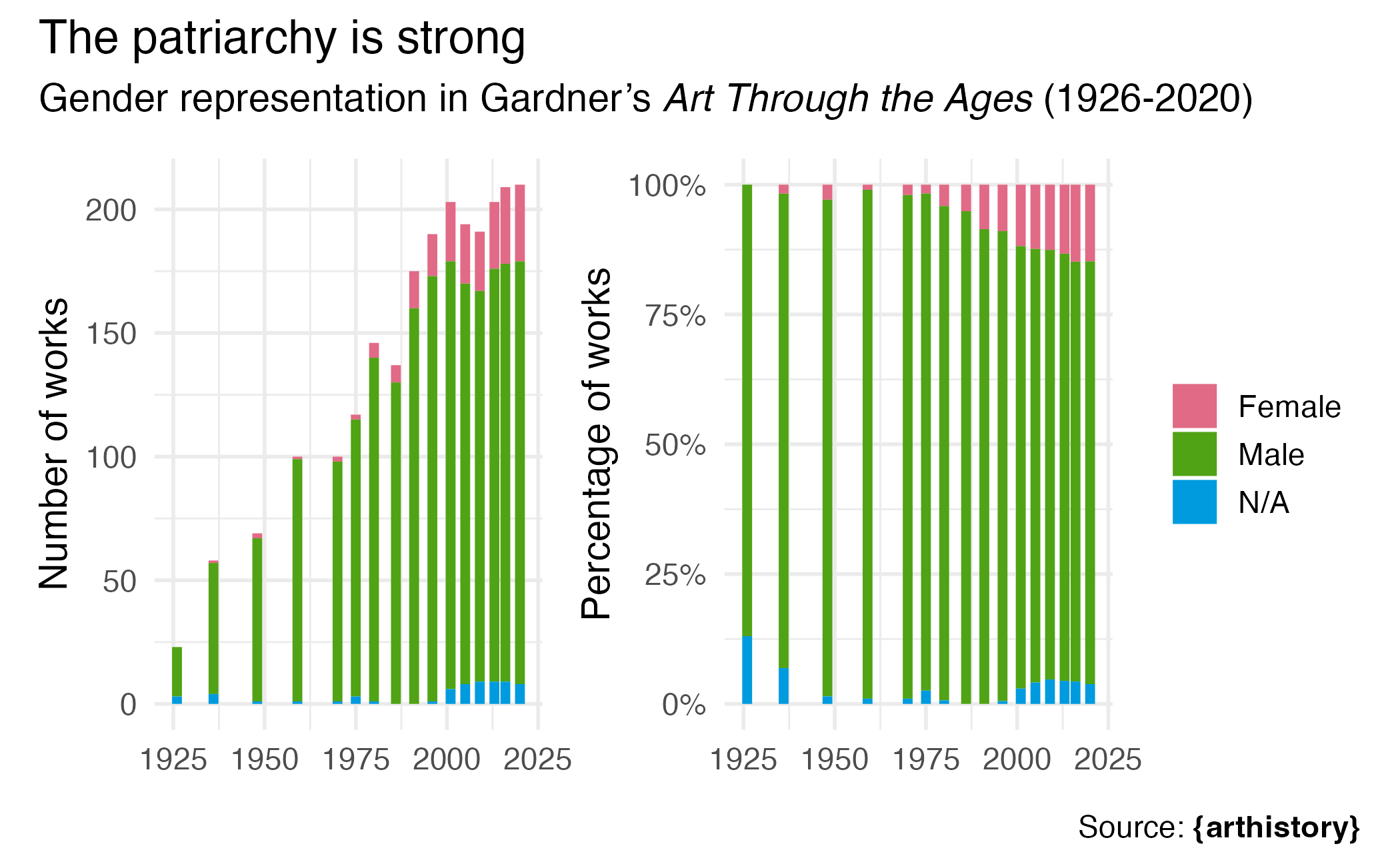

`ae-16`

Go to the course GitHub org and find your ae-16 (repo name will be suffixed with your GitHub name).
Clone the repo in RStudio Workbench, open the Quarto document in the repo, and follow along and complete the exercises.
Save, commit, and push your edits by the AE deadline – end of the day tomorrow.

Recap of AE

Generalized linear models allow us to fit models to predict non-continuous outcomes
Predicting binary outcomes requires modeling the log-odds of success, where p = probability of success
Interpreting logistic regression coefficients requires calculating predicted probabilities
Use training/test set splits to prevent overfitting
Use appropriate metrics to evaluate model performance
The decision threshold effects the predictions generated from a logistic regression model

Acknowledgments

Draws upon material from Data Science in a Box licensed under Creative Commons Attribution-ShareAlike 4.0 International

Lottery redux

Models for discrete outcomes

Announcements

Announcements

Goals

Predicting categorical data

Spam filters

Modelling spam

Modelling spam

Feel the Bern(oulli)

Framing the problem

Generalized linear models

Three characteristics of GLMs

Logistic regression

Logistic regression

Logit function, visualized

Properties of the logit

The logistic regression model

Modeling spam

Spam model

\(\Pr(\text{spam})\) for an email with 2000 characters

Sensitivity and specificity

False positive and negative

Sensitivity and specificity

Prediction

Goal: Building a spam filter

A multiple regression approach

Prediction

Underfitting and overfitting

Spending our data

Splitting data

Splitting data

Performing the split

Peek at the split

Modeling workflow

Fit a model to the training dataset

Categorical predictors

from and sent_email

Numerical predictors

Fit a model to the training dataset

Predict outcome on the testing dataset

Predict probabilities on the testing dataset

A closer look at predictions

Evaluate the performance

Evaluate the performance

Application exercise

Art history

ae-16

Recap of AE

Acknowledgments

Lottery redux

`from` and `sent_email`

`ae-16`