02:00
Hypothesis testing with randomization
Lecture 20
Dr. Benjamin Soltoff
Cornell University
INFO 2950 - Spring 2024
April 9, 2024
Announcements
Announcements
- Data collection/EDA feedback
- Midsemester feedback
- Roadmap rest of semester
Goals
- Hypothesis testing, p-values, and making conclusions
Test a claim about a population parameter
Use simulation-based methods to generate the null distribution
Calculate and interpret the p-value
Use the p-value to draw conclusions in the context of the data and the research question
- Identify one and two-tailed hypothesis tests
- Practice conducting and interpreting hypothesis tests
Hypothesis testing
Hypothesis testing
A hypothesis test is a statistical technique used to evaluate competing claims using data
Null hypothesis \(H_0\): An assumption about the population. “There is nothing going on.”
Alternative hypothesis, \(H_A\): A research question about the population. “There is something going on”.
Note: Hypotheses are always at the population level!
Confidence intervals vs. hypothesis testing
Related, but have distinct motivations
- Estimation \(\leadsto\) confidence interval
- Decision \(\leadsto\) hypothesis test
Vice consumption
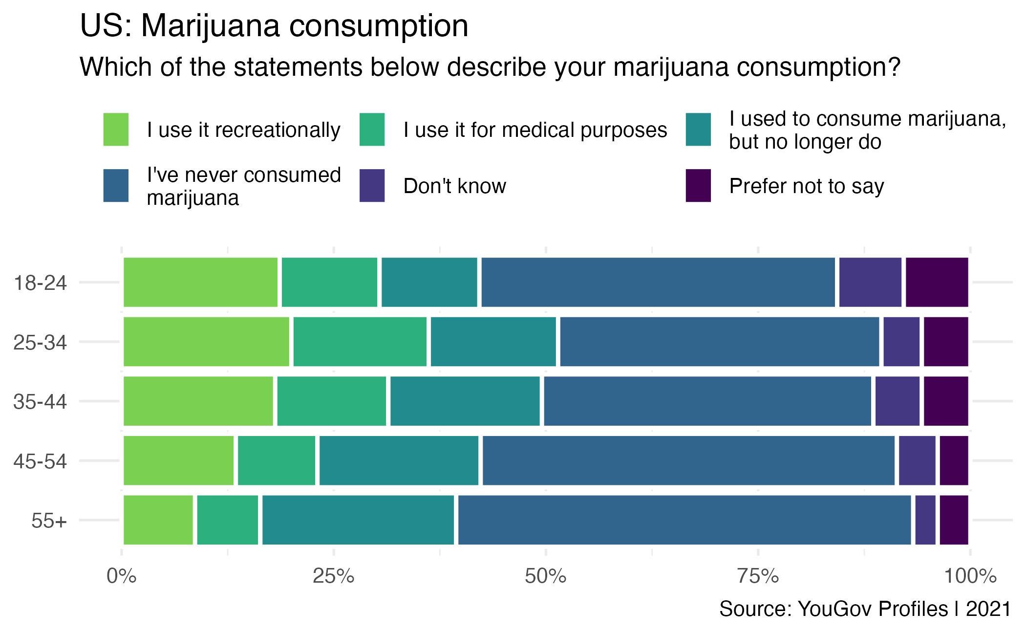
Writing hypotheses
As a researcher, you are interested in the average number of marijuana gummies consumed by Cornell students each week. An article on The Cornell Sun suggests that Cornell students consume, on average, 1.5 gummies each week. You are interested in evaluating if The Cornell Sun’s claim is too high. What are your hypotheses?
Writing hypotheses
As a researcher, you are interested in the average number of marijuana gummies Cornell students consume in a week.
An article on The Cornell Sun suggests that Cornell students consume, on average, 1.5 gummies each week. \(\rightarrow H_0: \mu = 1.5\)
You are interested in evaluating if The Cornell Sun’s estimate is too high. \(\rightarrow H_A: \mu < 1.5\)
Collecting data
Let’s suppose you manage to take a random sample of 1000 Cornell students and ask them how many gummies they consume and calculate the sample average to be \(\bar{x} = 1\).
Hypothesis testing “mindset”
Assume you live in a world where the null hypothesis is true: \(\mu = 1.5\).
Ask yourself how likely you are to observe the sample statistic, or something even more extreme, in this world: \(\Pr(\bar{x} < 1 | \mu = 1.5)\) = ?
Types of alternative hypotheses
- One sided (one tailed) alternatives: The parameter is hypothesized to be less than or greater than the null value, < or >
- Two sided (two tailed) alternatives: The parameter is hypothesized to be not equal to the null value, \(\ne\)
- Calculated as two times the tail area beyond the observed sample statistic
- More objective, and hence more widely preferred
An article on The Cornell Sun suggests that Cornell students consume, on average, 1.5 gummies each week. \(H_0: \mu = 1.5\)
Is The Cornell Sun’s estimate correct? (two sided) \(H_A: \mu \neq 1.5\)
Is The Cornell Sun’s estimate too high? (one sided) \(H_A: \mu < 1.5\)
Testing for independence
Is yawning contagious?
Do you think yawning is contagious?


Is yawning contagious?
An experiment conducted by the MythBusters tested if a person can be subconsciously influenced into yawning if another person near them yawns.
Study description
In this study 50 people were randomly assigned to two groups: 34 to a group where a person near them yawned (treatment) and 16 to a control group where they didn’t see someone yawn (control).
The data are in the openintro package: yawn
Proportion of yawners
# A tibble: 4 × 4
# Groups:   group [2]
  group result       n p_hat
  <fct> <fct>    <int> <dbl>
1 ctrl  not yawn    12 0.75
2 ctrl  yawn         4 0.25
3 trmt  not yawn    24 0.706
4 trmt yawn 10 0.294- Proportion of yawners in the treatment group: \(\frac{10}{34} = 0.2941\)
- Proportion of yawners in the control group: \(\frac{4}{16} = 0.25\)
- Difference: \(0.2941 - 0.25 = 0.0441\)
Independence?
Based on the proportions we calculated, do you think yawning is really contagious, i.e. are seeing someone yawn and yawning dependent?
# A tibble: 4 × 4
# Groups:   group [2]
  group result       n p_hat
  <fct> <fct>    <int> <dbl>
1 ctrl  not yawn    12 0.75
2 ctrl  yawn         4 0.25
3 trmt  not yawn    24 0.706
4 trmt  yawn        10 0.294
Dependence, or another possible explanation?
The observed differences might suggest that yawning is contagious, i.e. seeing someone yawn and yawning are dependent.
But the differences are small enough that we might wonder if they might simply be due to chance.
Perhaps if we were to repeat the experiment, we would see slightly different results.
So we will do just that - well, somewhat - and see what happens.
Instead of actually conducting the experiment many times, we will simulate our results.
Two competing claims
Null hypothesis: “There is nothing going on.”
Yawning and seeing someone yawn are independent, yawning is not contagious, observed difference in proportions is simply due to chance.
\[H_0: p_{\text{treatment}} - p_{\text{control}} = 0\]
Alternative hypothesis: “There is something going on.” Yawning and seeing someone yawn are dependent, yawning is contagious, observed difference in proportions is not due to chance.
\[H_a: p_{\text{treatment}} - p_{\text{control}} \neq 0\]
Running the randomization
- Randomly shuffle the rows in the data frame.
- Split off the first 16 rows and set them aside. These rows represent the people in the control group.
- Split off the final 34 rows and set them aside. These rows represent the people in the treatment group.
- Calculate the proportion of people in the control group who yawned. Calculate the proportion of people in the treatment group who yawned.
- Calculate the difference in proportions of yawners (treatment - control) and plot it on the chart.
Simulation by computation
Simulation by computation
- Start with the data frame
- Specify the variables
- Since the response variable is categorical, specify the level which should be considered as “success”
Simulation by computation
- Start with the data frame
- Specify the variables
- State the null hypothesis (yawning and whether or not you see someone yawn are independent)
Simulation by computation
- Start with the data frame
- Specify the variables
- State the null hypothesis
- Generate simulated differences via randomization
Simulation by computation
- Start with the data frame
- Specify the variables
- State the null hypothesis
- Generate simulated differences via randomization
- Calculate the sample statistic of interest (difference in proportions)
- Since the explanatory variable is categorical, specify the order in which the subtraction should occur for the calculation of the sample statistic, \((\hat{p}_{\text{treatment}} - \hat{p}_{\text{control}})\).
Simulation by computation
- Save the result
- Start with the data frame
- Specify the variables
- State the null hypothesis
- Generate simulated differences via permutation
- Calculate the sample statistic of interest
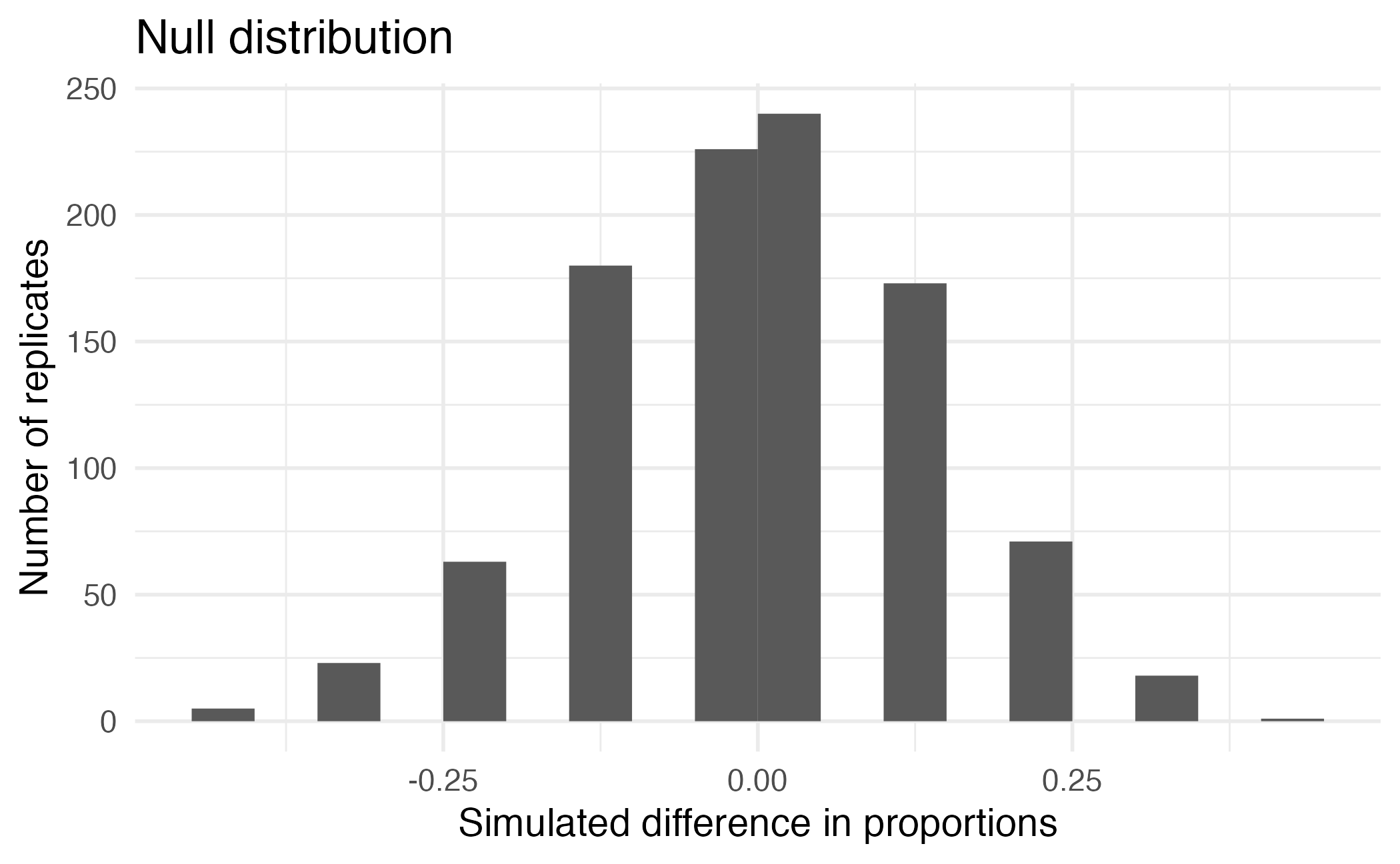
Visualizing the null distribution
What would you expect the center of the null distribution to be?
Calculating the p-value, visually
What is the p-value, i.e. in what % of the simulations was the simulated difference in sample proportion at least as extreme as the observed difference in sample proportions?
Calculating the p-value, directly
Significance level
We often use 5% as the cutoff for whether the p-value is low enough that the data are unlikely to have come from the null model. This cutoff value is called the significance level, \(\alpha\).
If p-value < \(\alpha\), reject \(H_0\) in favor of \(H_A\): The data provide convincing evidence for the alternative hypothesis.
If p-value > \(\alpha\), fail to reject \(H_0\) in favor of \(H_A\): The data do not provide convincing evidence for the alternative hypothesis.
The p-value should be set in advance based on your concern of making a false positive (reject the null hypothesis when in fact it is correct) vs. false negative (fail to reject the null hypothesis when in fact it is incorrect).
Scientists are typically most concerned with avoiding false positives and set a significance level of \(\alpha = 0.05\).
Conclusion
What is the conclusion of the hypothesis test?
Do you “buy” this conclusion?
Inference with mathematical models
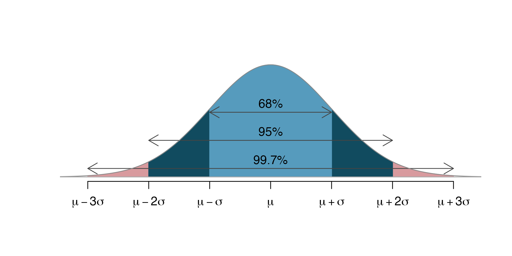
Central limit theorem
- Assumes sampling statistics adhere to a normal distribution
- Relies on the Central Limit Theorem and key assumptions
- Observations in the sample are independent
- The sample size is sufficiently large
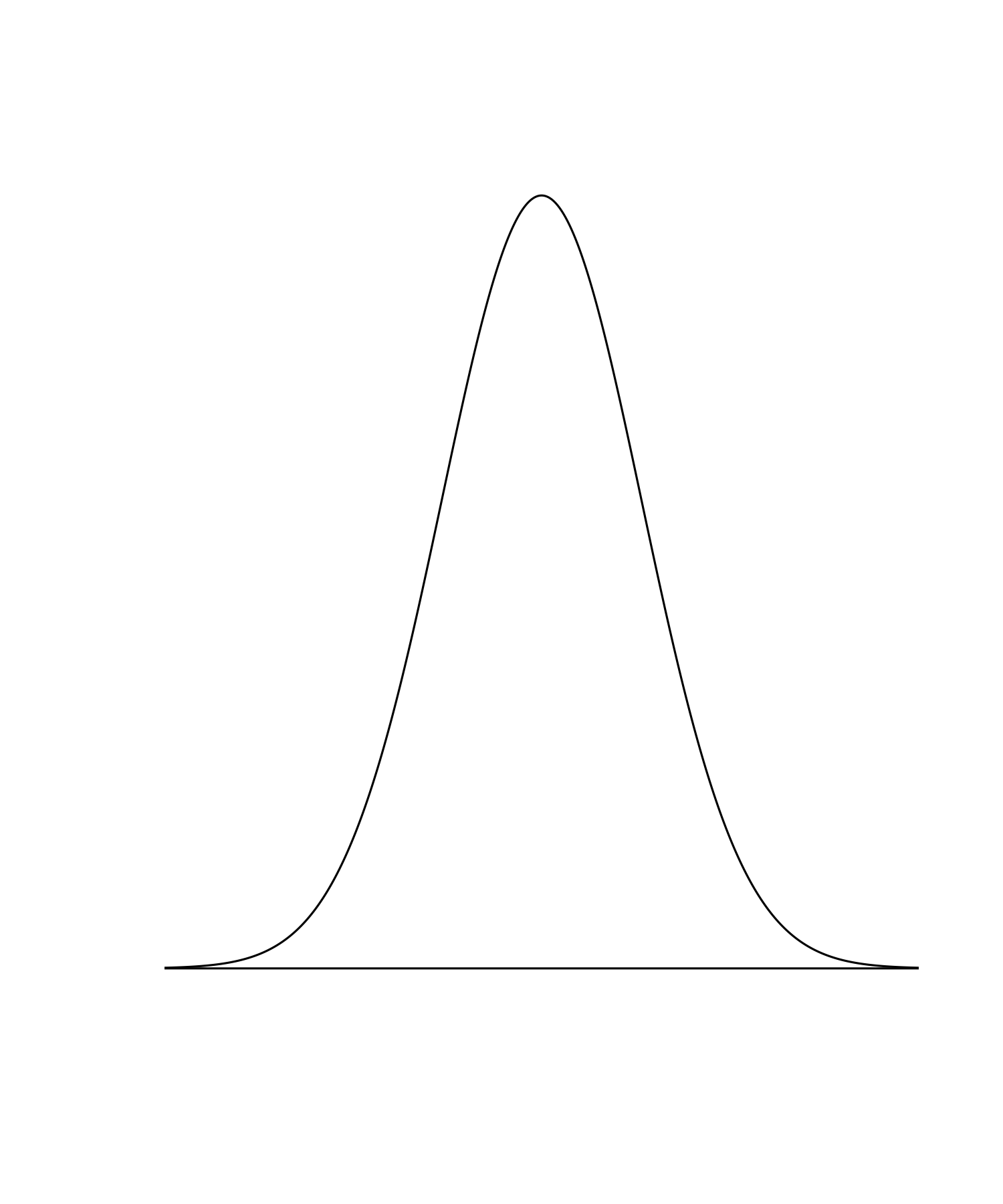
Inference with the Normal Distribution
Application exercise
[OC] If You Order Chipotle Online, You Are Probably Getting Less Food
byu/G_NC indataisbeautiful
ae-18
- Go to the course GitHub org and find your
ae-18(repo name will be suffixed with your GitHub name). - Clone the repo in RStudio Workbench, open the Quarto document in the repo, and follow along and complete the exercises.
- Save, commit, and push your edits by the AE deadline – end of the day tomorrow.
Recap of AE
- Hypothesis tests are used to evaluate competing claims using data
- The p-value is the probability of observing a test statistic as extreme as the one computed from the sample data, assuming the null hypothesis is true
- The significance level is the probability of rejecting the null hypothesis when it is true
- Permutation-based approaches use repeated simulations to estimate the distribution of the test statistic under the null hypothesis
Acknowledgments
- Draws upon material from Data Science in a Box licensed under Creative Commons Attribution-ShareAlike 4.0 International
Total Eclipse of the Clouds