# A tibble: 2 × 5
  term              estimate std.error statistic   p.value
  <chr>                <dbl>     <dbl>     <dbl>     <dbl>
1 (Intercept)        -5781.     306.       -18.9 5.59e- 55
2 flipper_length_mm 49.7 1.52 32.7 4.37e-107Quantifying uncertainty with bootstrap intervals
Lecture 21
April 11, 2024
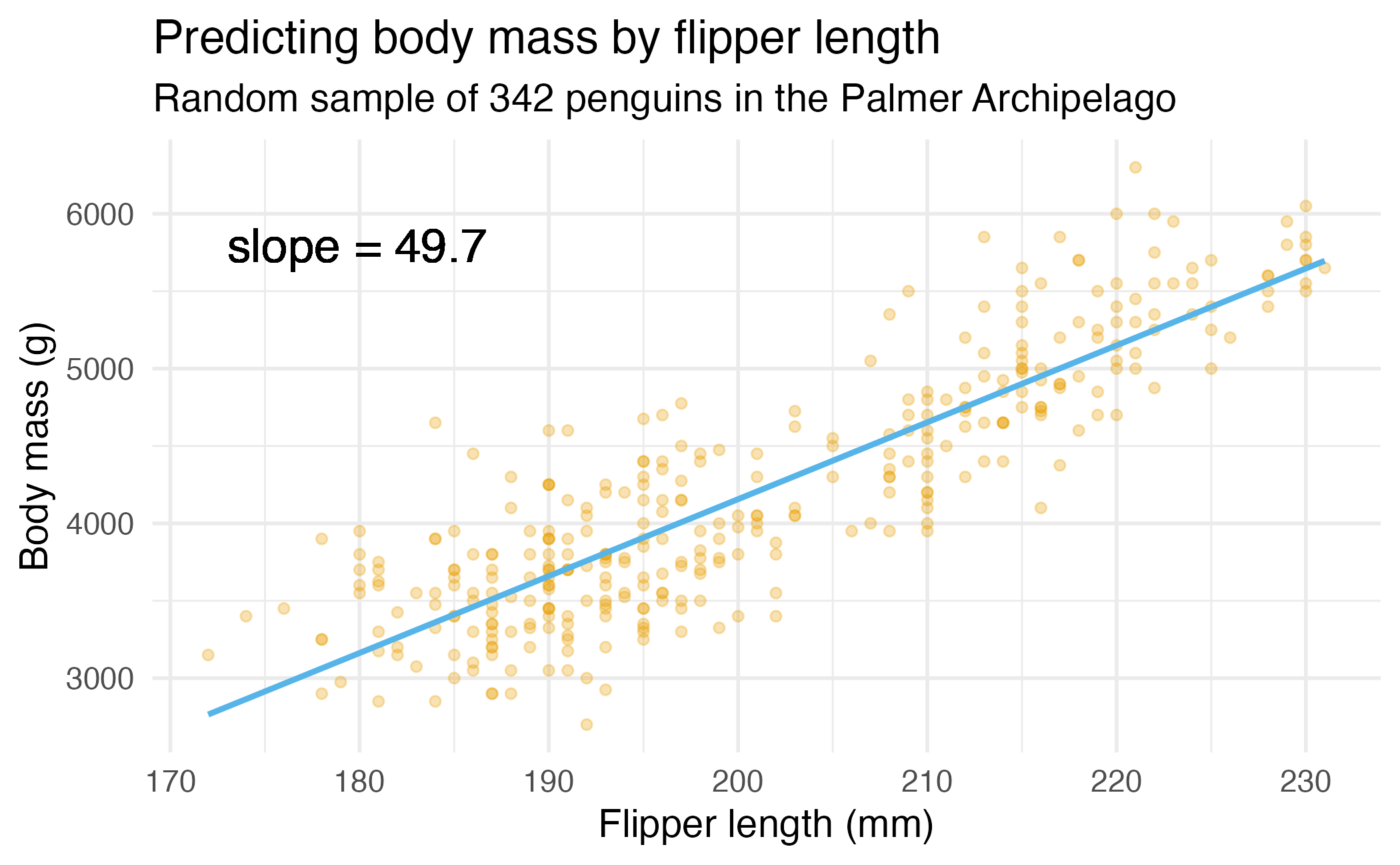
Remember the penguins
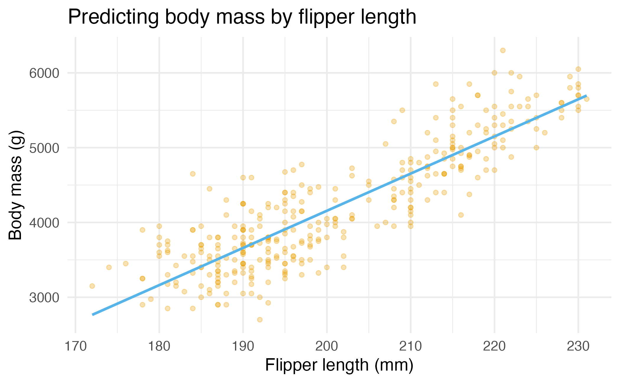
\[ \widehat{\text{body mass}} = -5781 + 49.7 \times \text{flipper length} \]
What does this line tell us?
If you want to catch a fish, do you prefer a spear or a net?


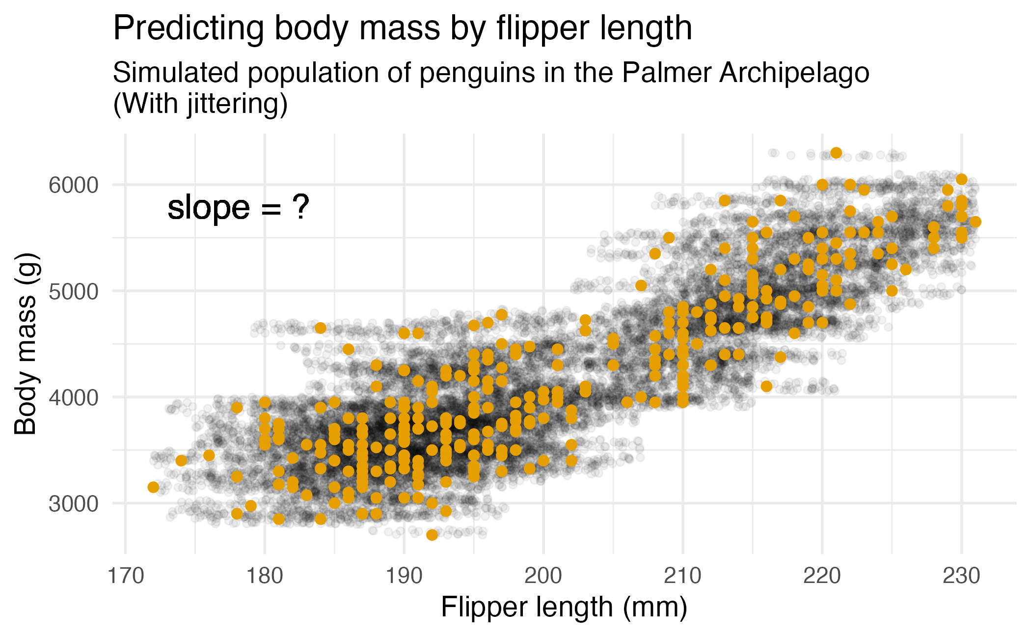
Observed sample
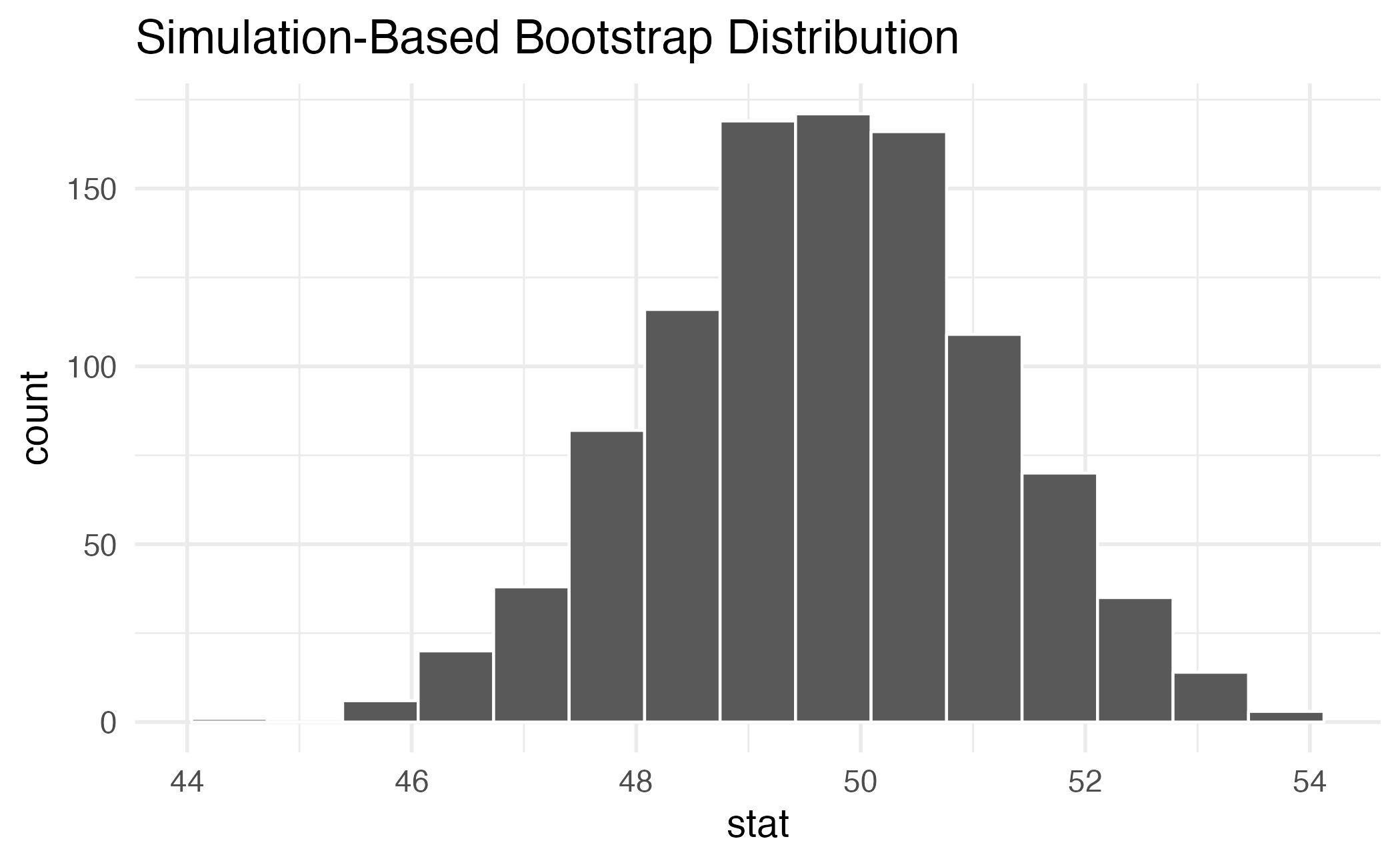
Bootstrap population
Generated assuming there are more penguins like the ones in the observed sample…

Random sampling
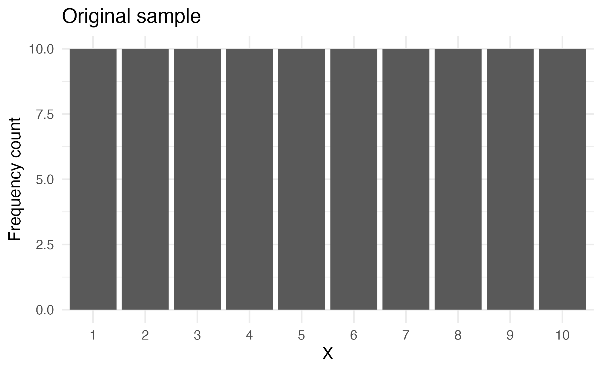
Sampling without replacement
Sampling with replacement
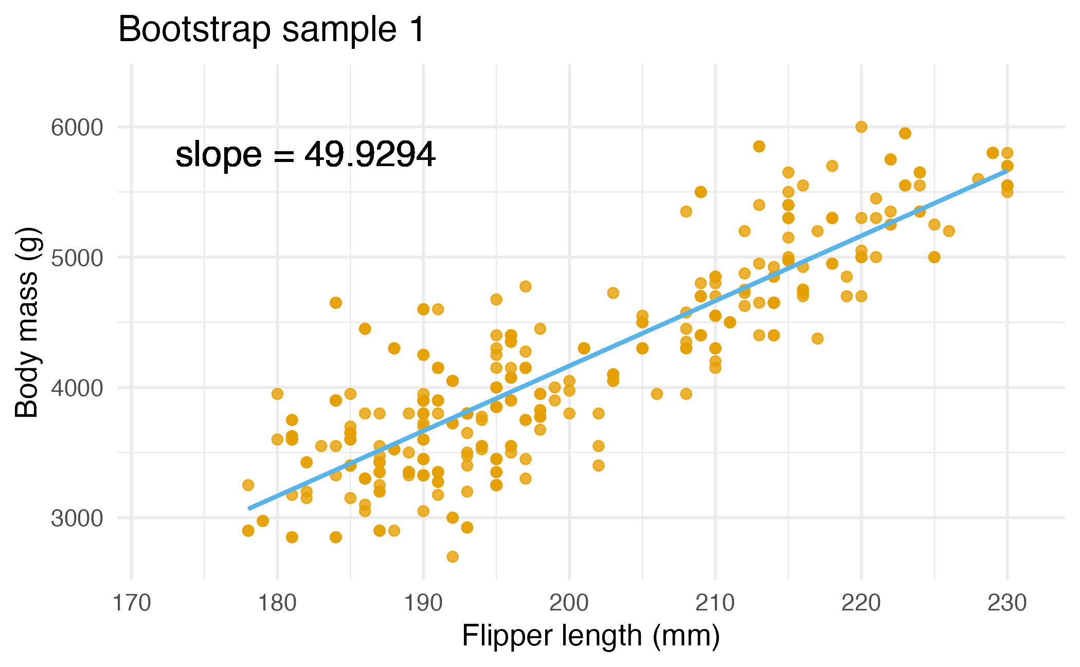
Bootstrap sample 1
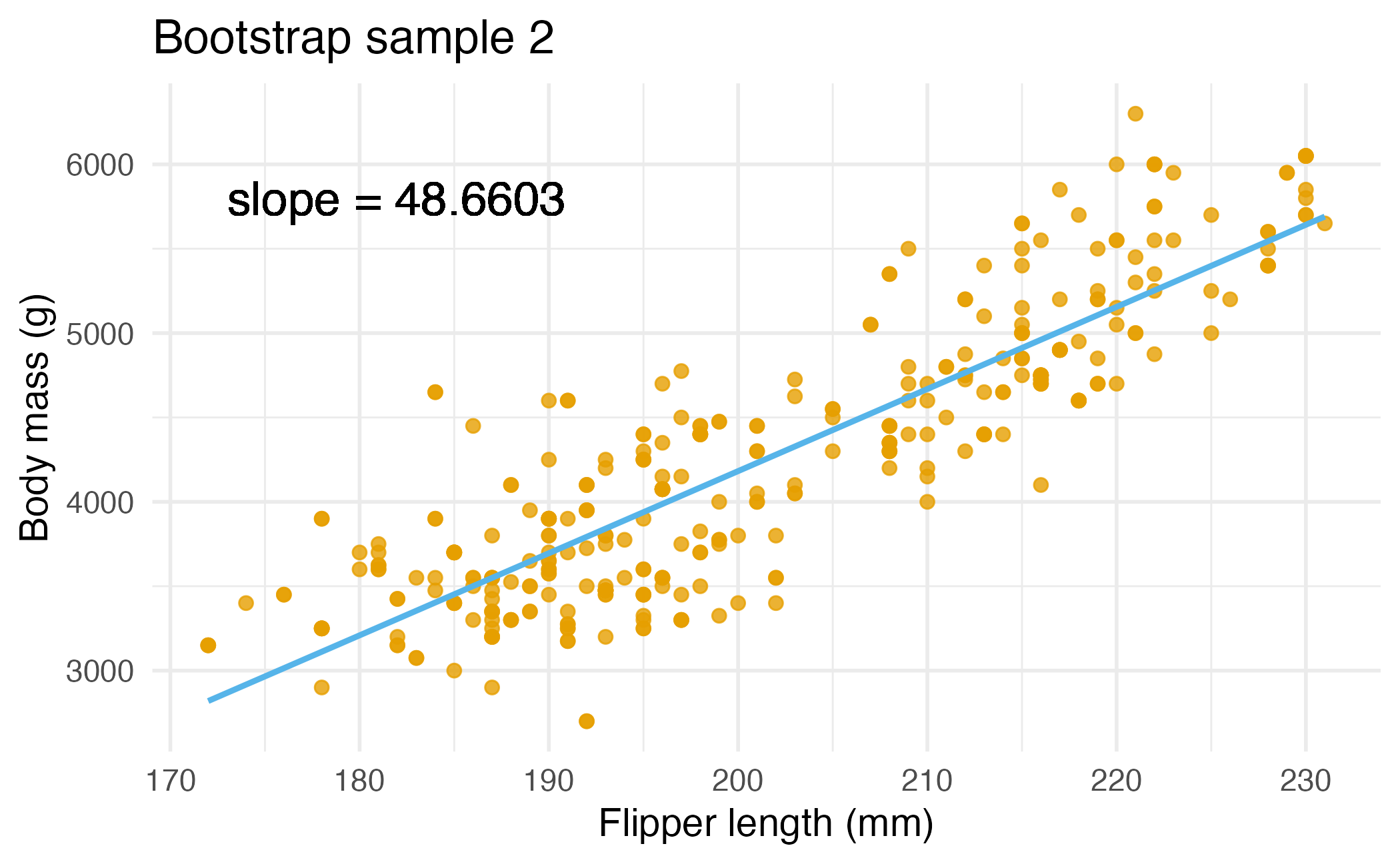
Bootstrap sample 2
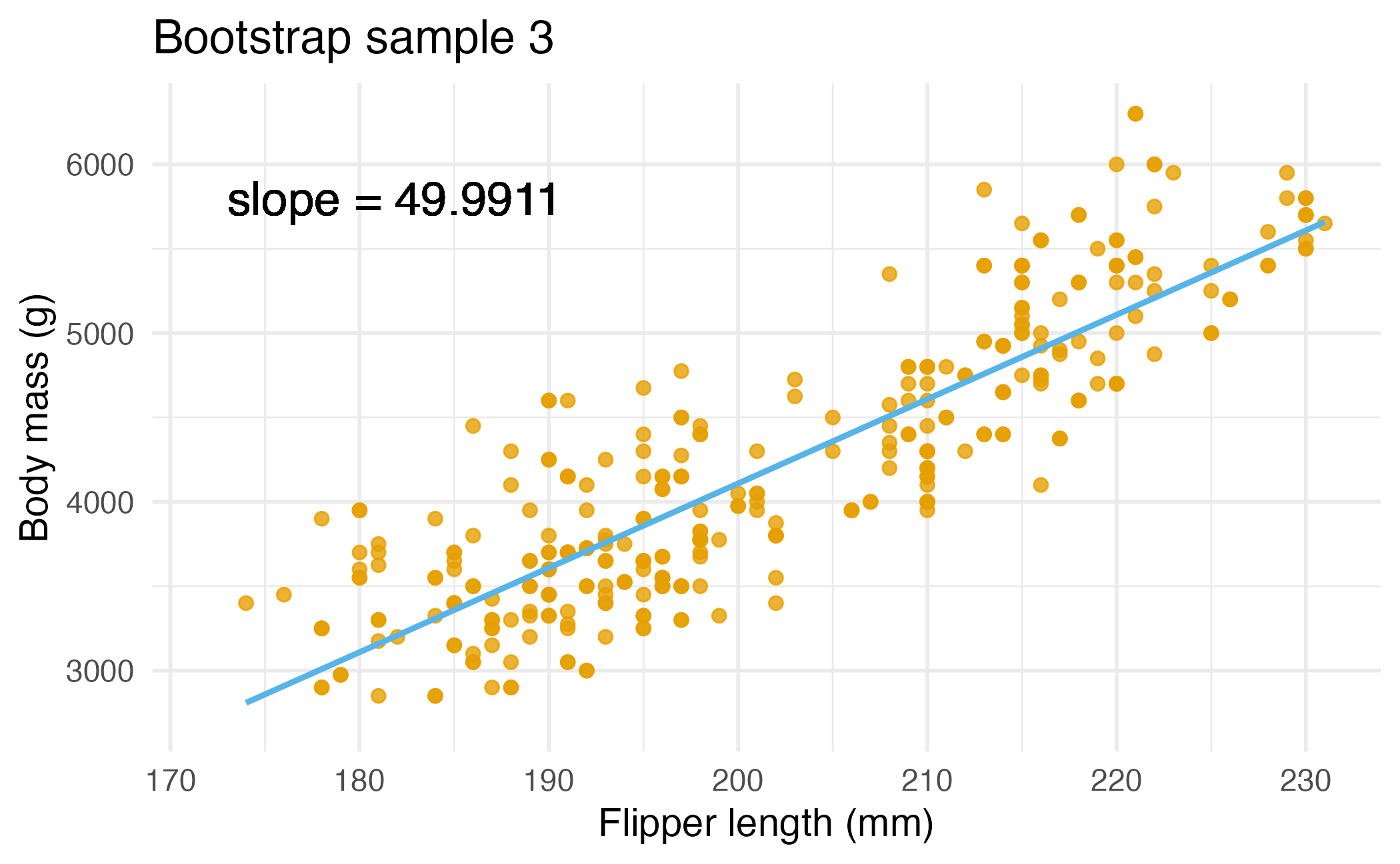
Bootstrap sample 3
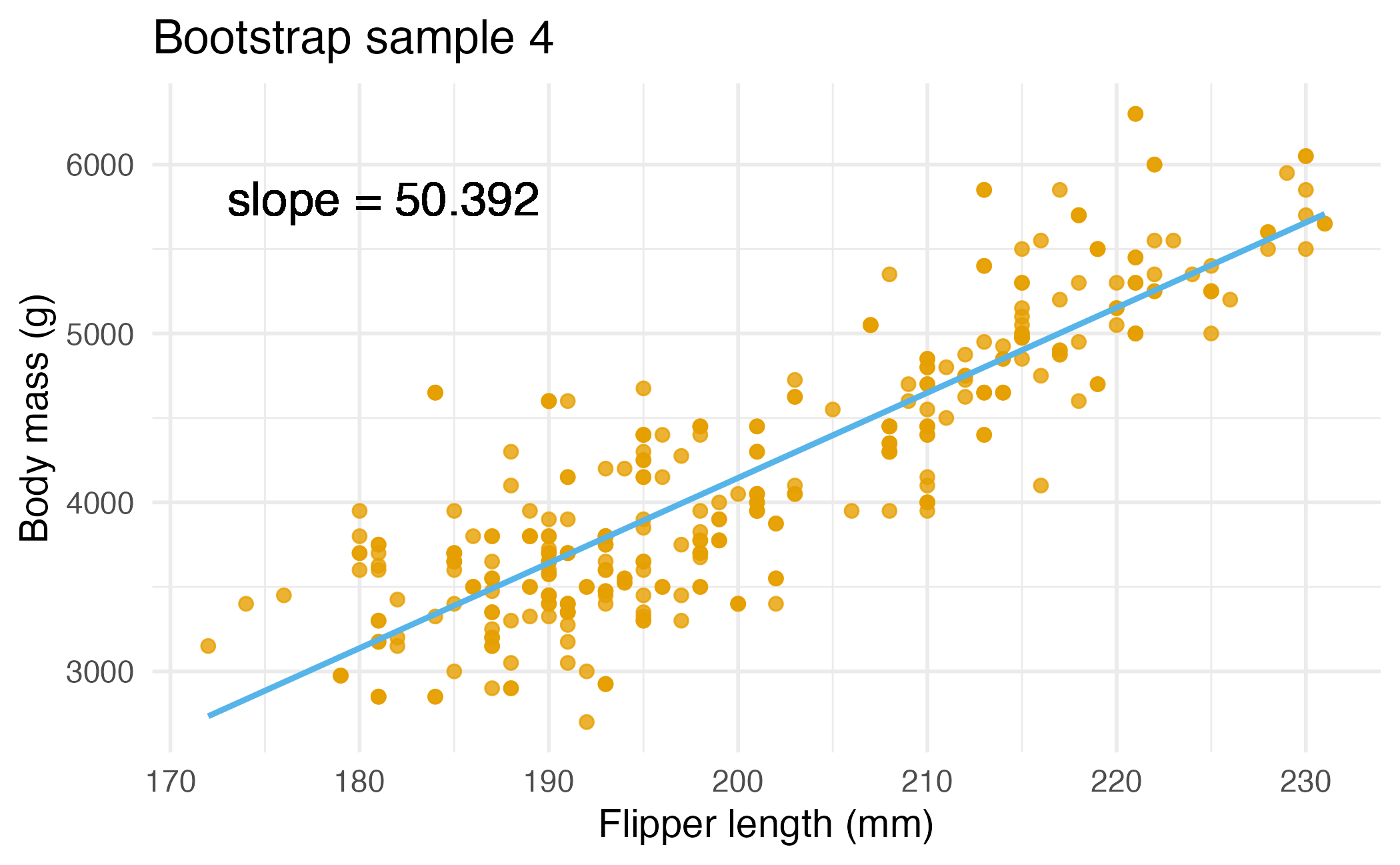
Bootstrap sample 4
Bootstrap samples 1 - 4
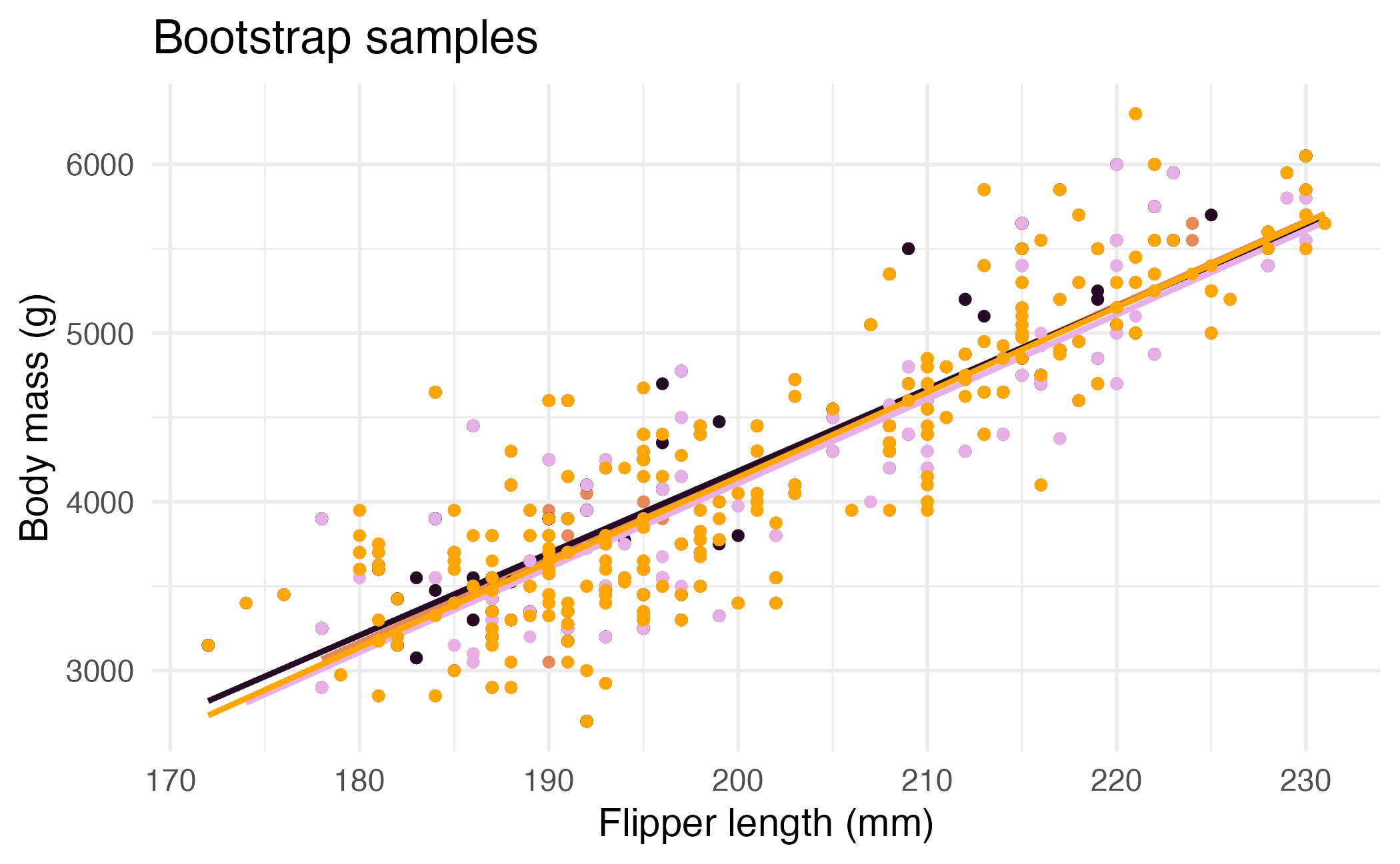
Many many samples…
Slopes of bootstrap samples
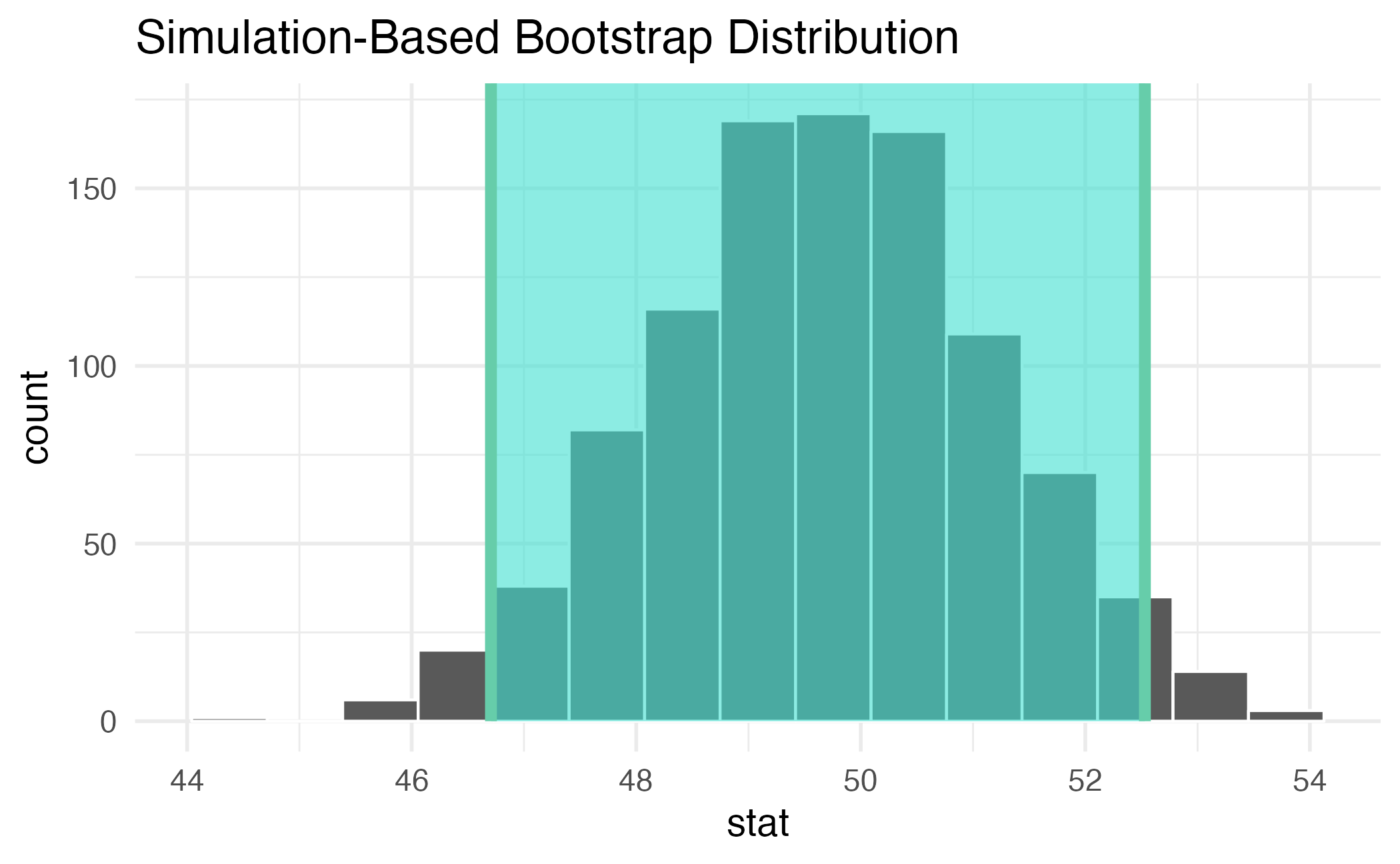
95% confidence interval
Confidence level
We are 95% confident that …
- Suppose we took many samples from the original population and built a 95% confidence interval based on each sample.
- Then about 95% of those intervals would contain the true population parameter.
Confidence intervals identify a plausible range of values for the population parameter…
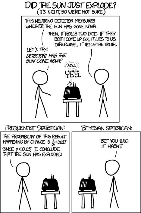
…they do not identify the probability that the true population parameter falls within the specified range.
Commonly used confidence intervals
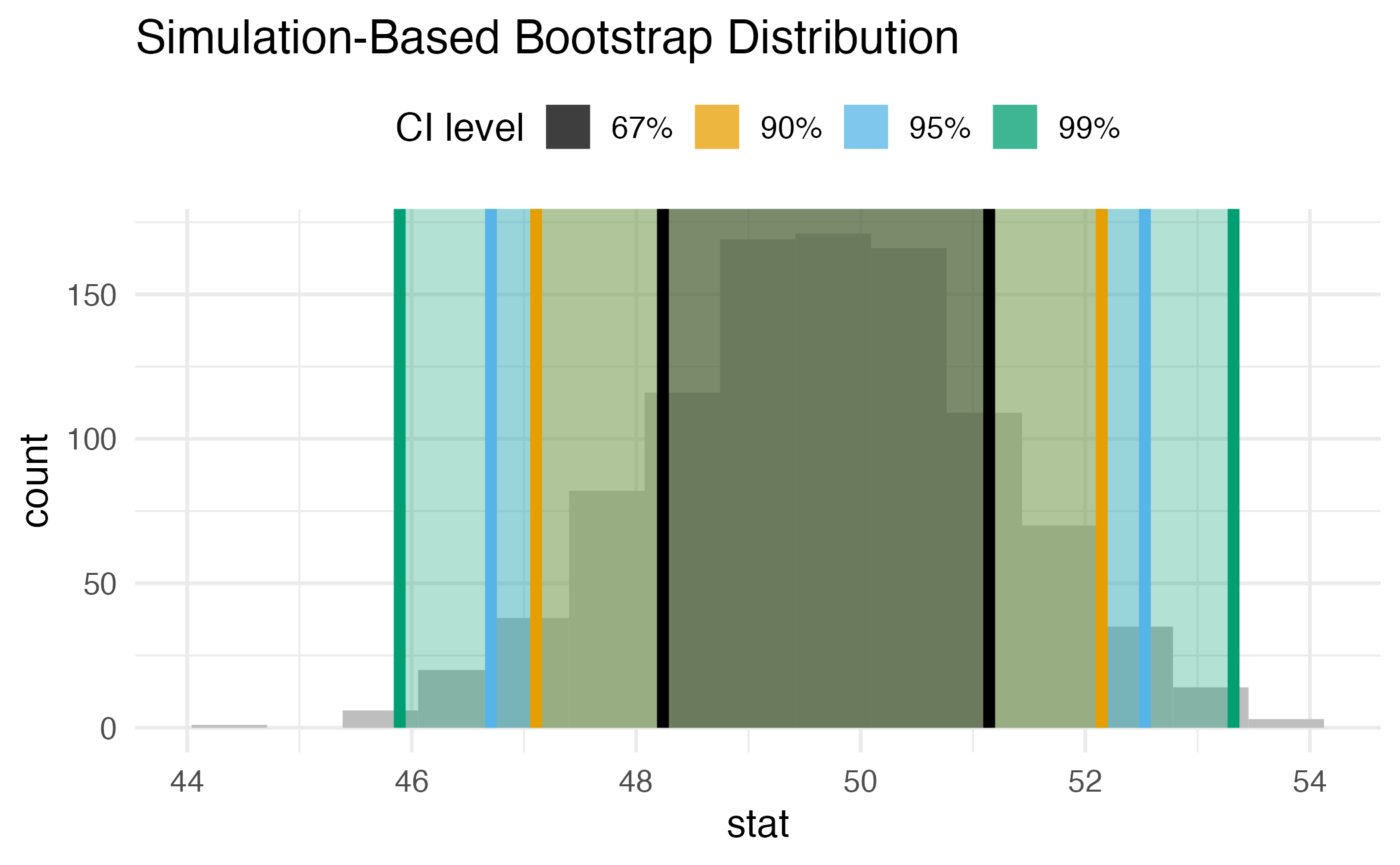
Precision vs. accuracy
If we want to be very certain that we capture the population parameter, should we use a wider or a narrower interval? What drawbacks are associated with using a wider interval?

How can we get best of both worlds – high precision and high accuracy?
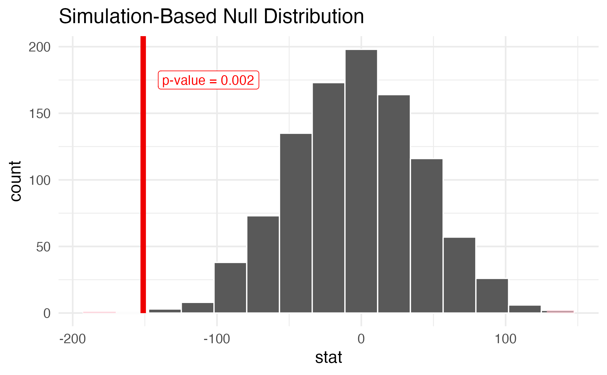
Hypothesis test
# A tibble: 1 × 1
  p_value
    <dbl>
1   0.026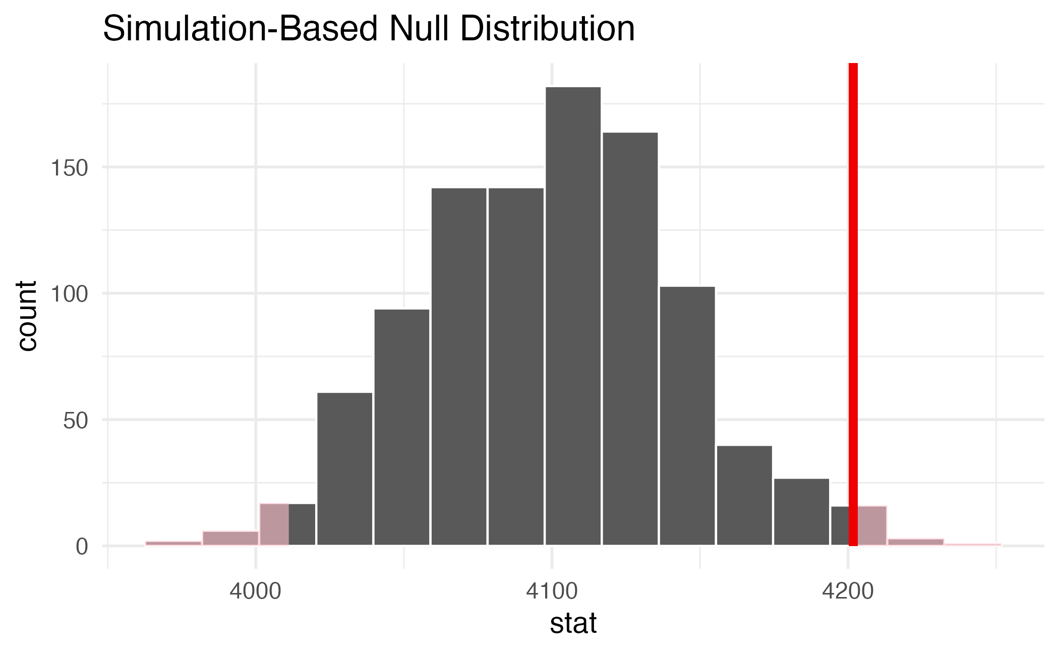
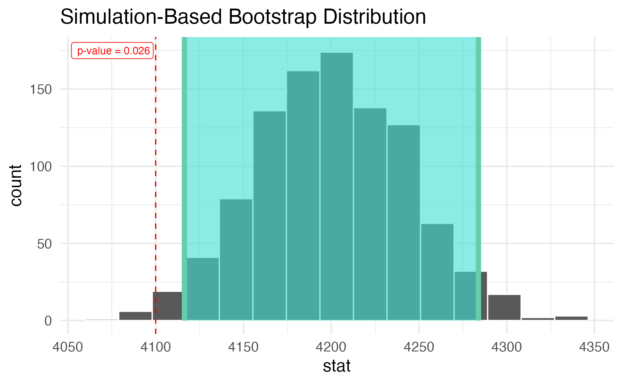
95% confidence interval
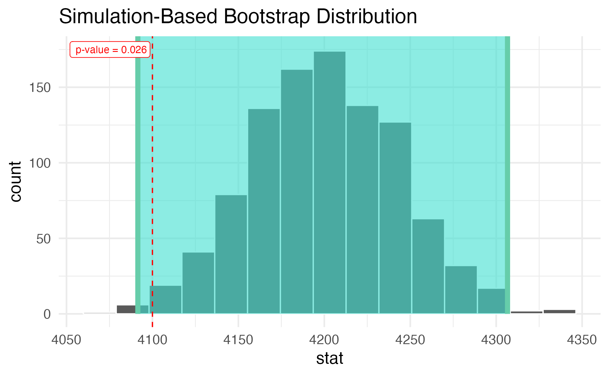
99% confidence interval
Math (and unit conversion) is hard
Corrected null hypothesis test
Bought a car