library(tidymodels)
## ── Attaching packages ────────────────────────────────────── tidymodels 1.1.1 ──
## ✔ broom        1.0.5     ✔ rsample      1.2.0
## ✔ dials        1.2.0     ✔ tune         1.1.2
## ✔ infer        1.0.5     ✔ workflows    1.1.4
## ✔ modeldata    1.2.0     ✔ workflowsets 1.0.1
## ✔ parsnip      1.2.0     ✔ yardstick    1.3.0
## ✔ recipes      1.0.9
## ── Conflicts ───────────────────────────────────────── tidymodels_conflicts() ──
## ✖ scales::discard() masks purrr::discard()
## ✖ dplyr::filter()   masks stats::filter()
## ✖ recipes::fixed()  masks stringr::fixed()
## ✖ dplyr::lag()      masks stats::lag()
## ✖ yardstick::spec() masks readr::spec()
## ✖ recipes::step()   masks stats::step()
## • Use suppressPackageStartupMessages() to eliminate package startup messagesIntroduction to machine learning
Lecture 22
Dr. Benjamin Soltoff
Cornell University
INFO 2950 - Spring 2024
April 16, 2024
Announcements
Announcements
- Exam 02 (final exam) accommodations
- Homework 06
- Preregistration of analyses
Application exercise
ae-20
- Go to the course GitHub org and find your
ae-20(repo name will be suffixed with your GitHub name). - Clone the repo in RStudio Workbench, open the Quarto document in the repo, and follow along and complete the exercises.
- Render, commit, and push your edits by the AE deadline – end of tomorrow
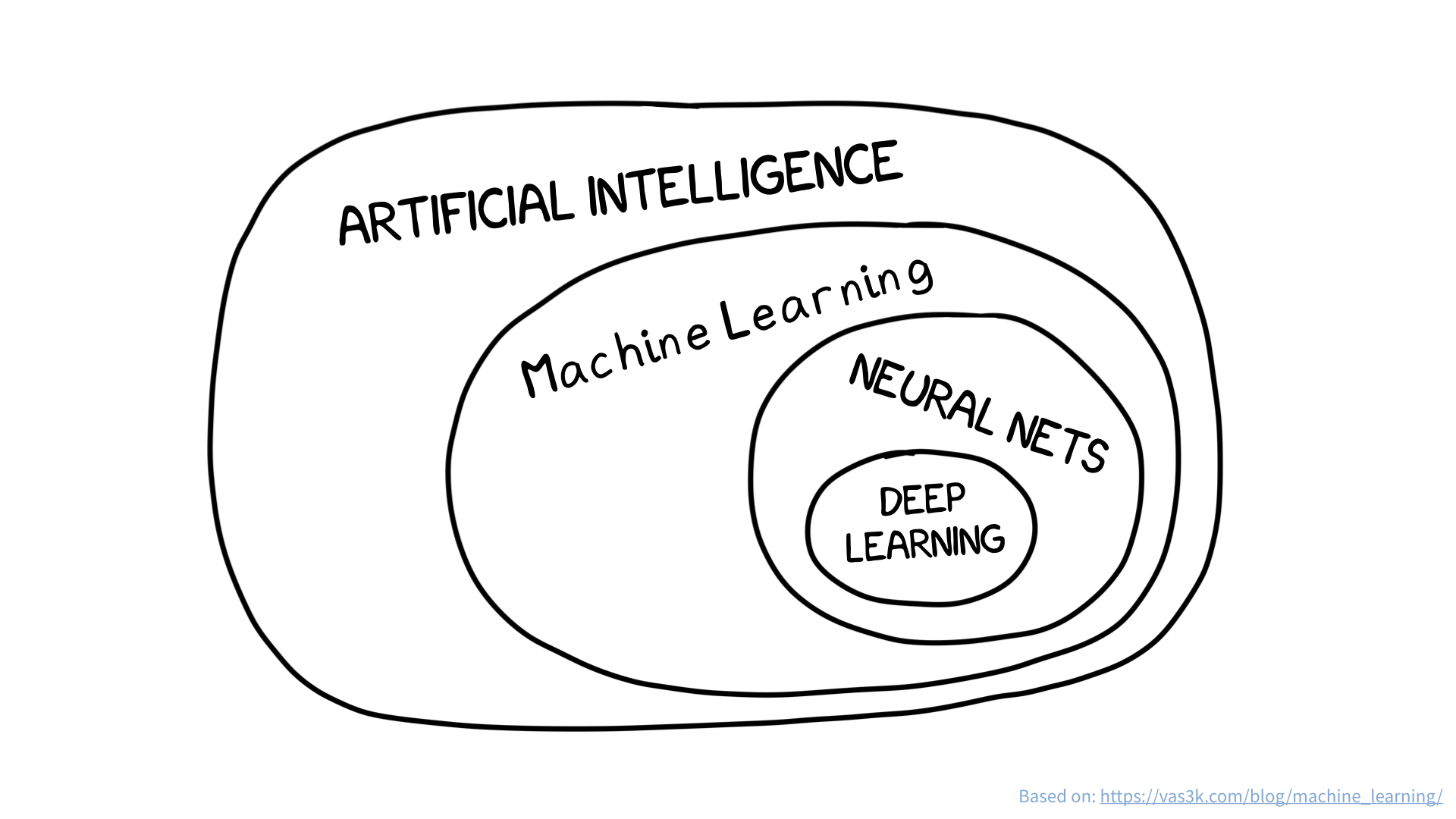
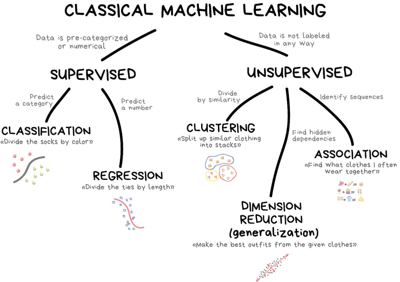
What is machine learning?


Examples of supervised learning
- Will a user click on this ad?
- Will a police officer engage in misconduct in the next six months?
- How many individuals will become infected with COVID-19 in the next week?
Two modes
Classification
Will this home sell in the next 30 days?
Regression
What will the sale price be for this home?
Two cultures
Statistics
- model first
- inference emphasis
Machine Learning
- data first
- prediction emphasis
Statistics
“Statisticians, like artists, have the bad habit of falling in love with their models.”
— George Box
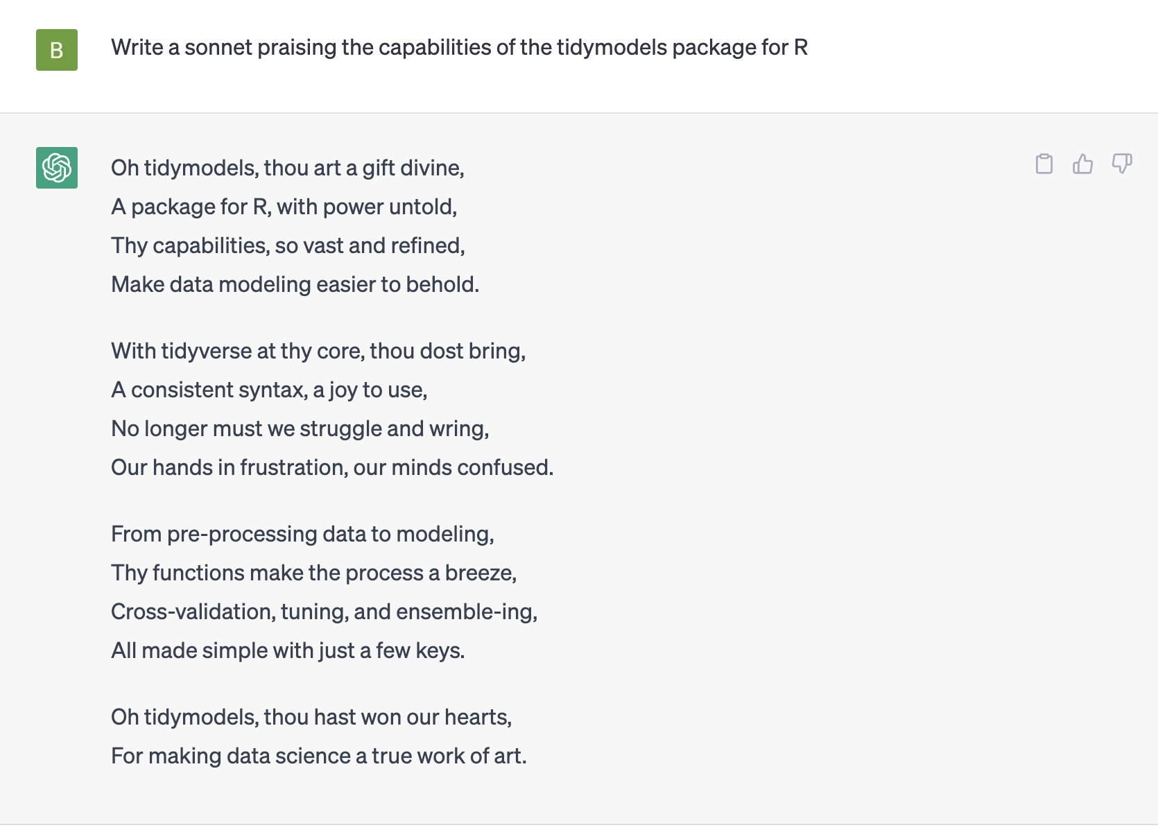
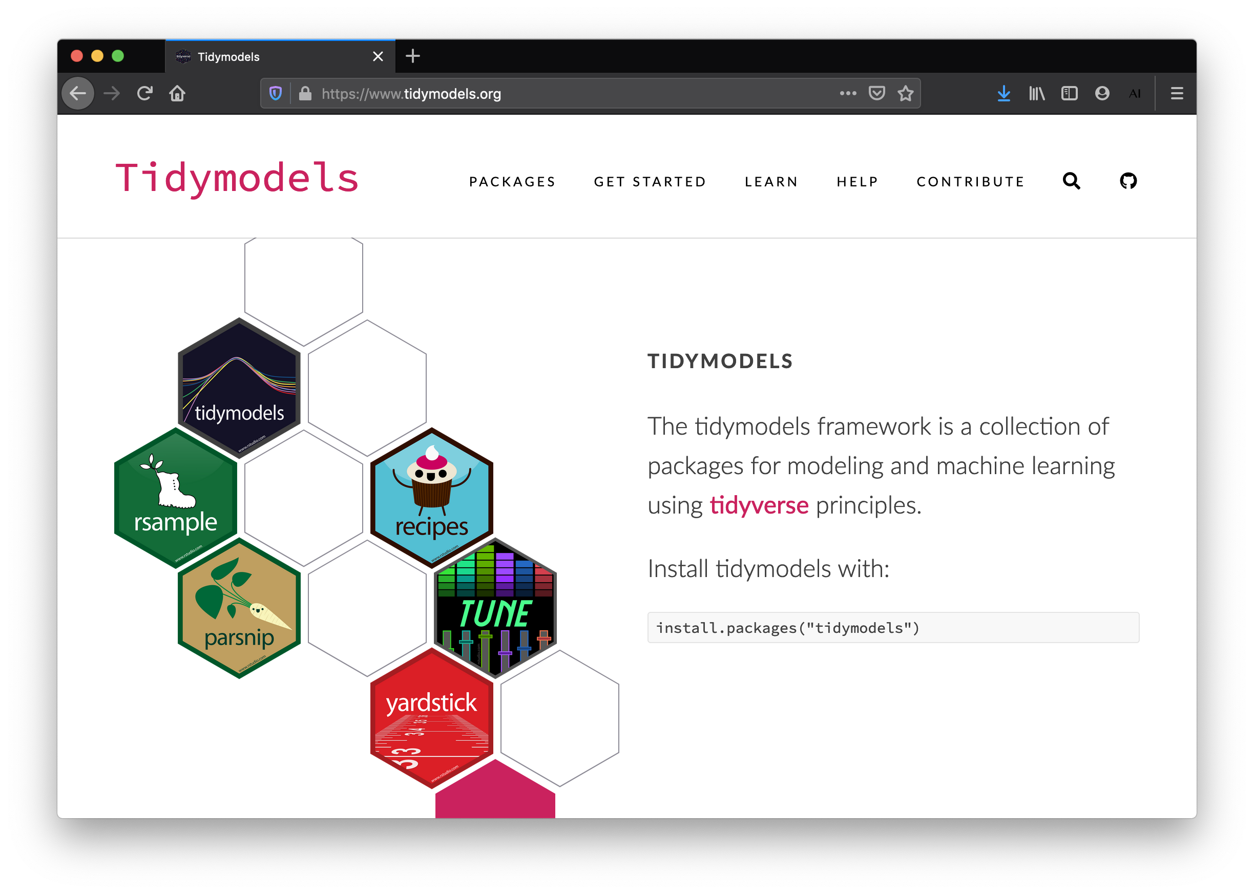
tidymodels
tidymodels
Predictive modeling
Children at hotels

Hotel booking demand
Hotel booking demand
- N = 4000
- 1 categorical outcome:
children - 21 predictors

What is the goal of machine learning?
Build models that
generate accurate predictions
for future, yet-to-be-seen data.
🔨 Build models with parsnip
parsnip
To specify a model with parsnip
- Pick a model
- Set the engine
- Set the mode (if needed)
Provides a unified interface to many models, regardless of the underlying package.
To specify a model with parsnip
To specify a model with parsnip
To specify a model with parsnip
1. Pick a model
All available models are listed at
https://www.tidymodels.org/find/parsnip/
logistic_reg()
Specifies a model that uses logistic regression
logistic_reg()
Specifies a model that uses logistic regression
set_engine()
Adds an engine to power or implement the model.
set_mode()
Sets the class of problem the model will solve, which influences which output is collected. Not necessary if mode is set in Step 1.
⏱️ Your turn 1
Run the chunk in your .qmd and look at the output. Then, copy/paste the code and edit to create:
a decision tree model for classification
that uses the
C5.0engine.
Save it as tree_mod and look at the object. What is different about the output?
Hint: you’ll need https://www.tidymodels.org/find/parsnip/
03:00
Now we’ve built a model.
But, how do we use a model?
First - what does it mean to use a model?

Statistical models learn from the data.
Many learn model parameters, which can be useful as values for inference and interpretation.
fit()
Train a model by fitting a model. Returns a parsnip model fit.
fit()
Train a model by fitting a model. Returns a parsnip model fit.
A fitted model
lr_mod |>
  fit(children ~ average_daily_rate + stays_in_weekend_nights,
    data = hotels
  ) |>
  broom::tidy()
## # A tibble: 3 × 5
##   term                estimate std.error statistic   p.value
##   <chr>                  <dbl>     <dbl>     <dbl>     <dbl>
## 1 (Intercept)           2.06    0.0956       21.5  5.31e-103
## 2 average_daily_rate   -0.0168  0.000710    -23.7  9.78e-124
## 3 stays_in_weekend_n…  -0.0671  0.0352       -1.91 5.63e-  2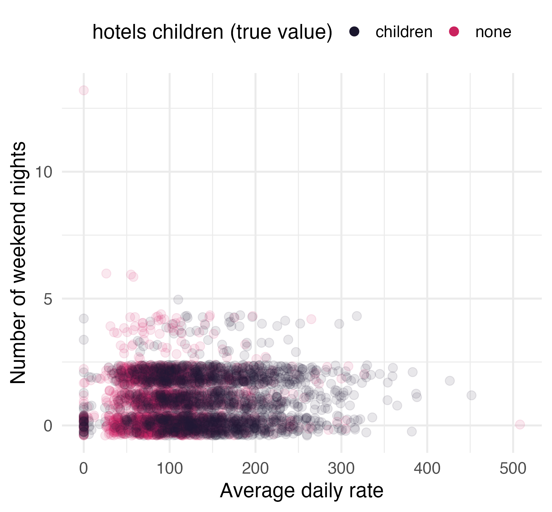
“All models are wrong, but some are useful”
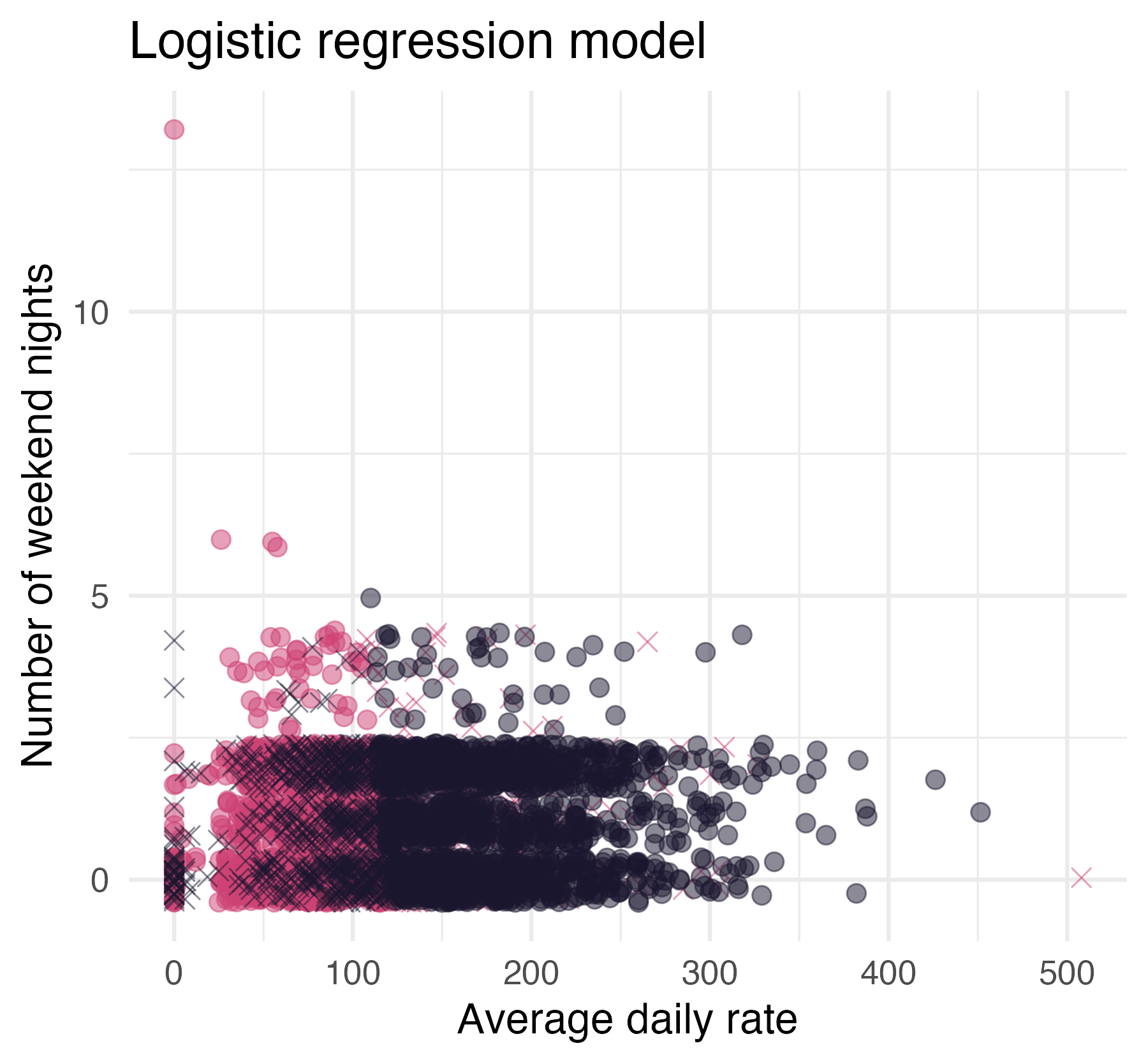
##           Truth
## Prediction children none
##   children     1277  483
##   none          723 1517
“All models are wrong, but some are useful”
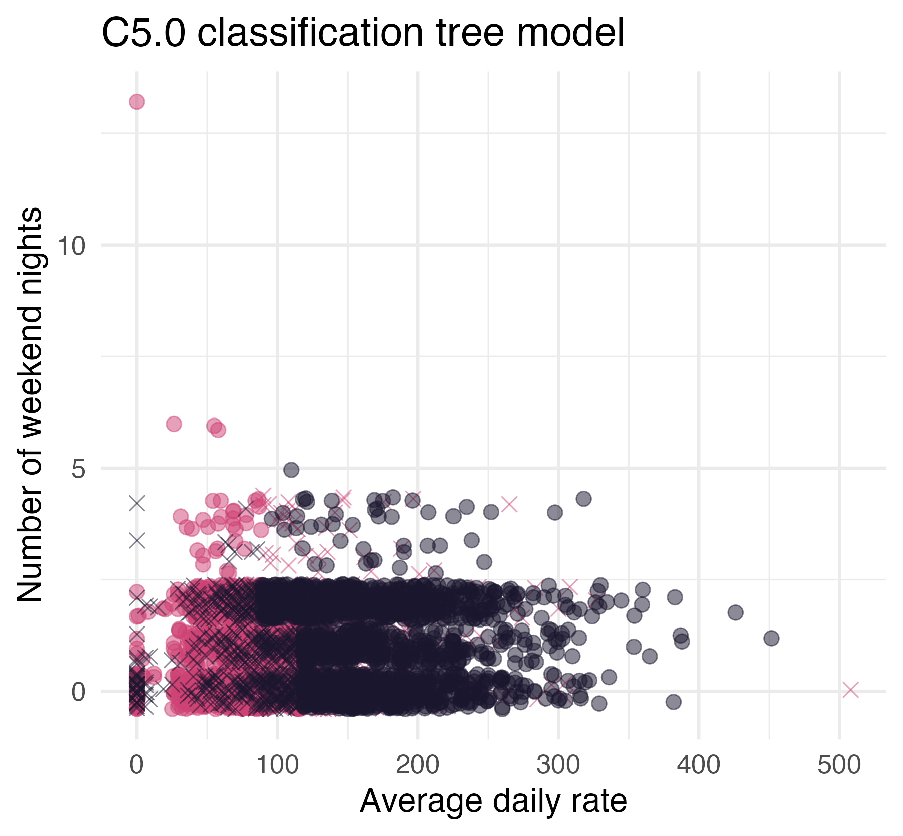
##           Truth
## Prediction children none
##   children     1446  646
##   none          554 1354
Axiom
The best way to measure a model’s performance at predicting new data is to predict new data.
♻️ Resample models with rsample
rsample
The holdout method
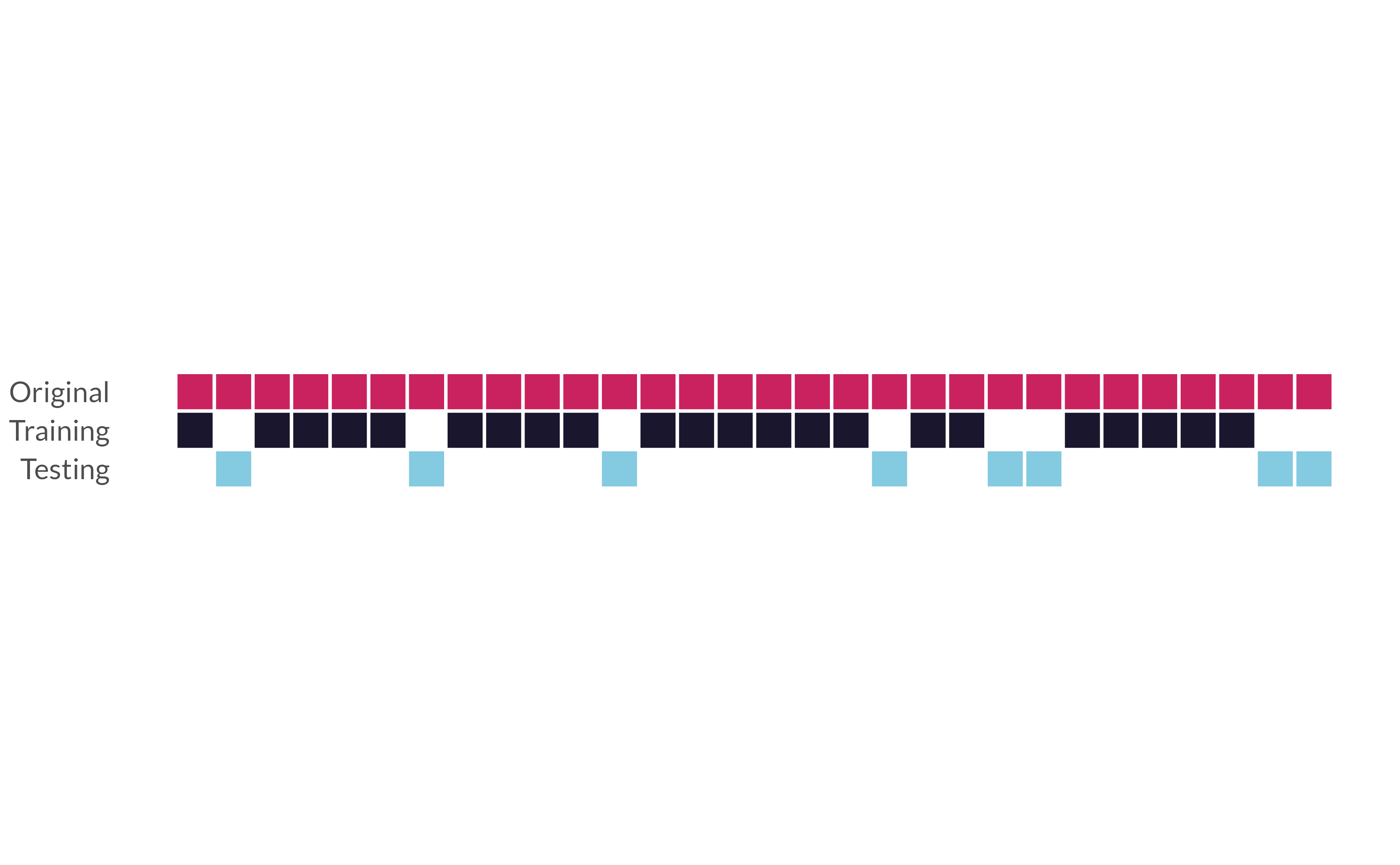
initial_split()*
“Splits” data randomly into a single testing and a single training set.
initial_split()
training() and testing()*
Extract training and testing sets from an rsplit
training()
hotels_train <- training(hotels_split)
hotels_train
## # A tibble: 3,000 × 22
##    hotel        lead_time stays_in_weekend_nights
##    <fct>            <dbl>                   <dbl>
##  1 City_Hotel          65                       1
##  2 City_Hotel           0                       2
##  3 Resort_Hotel       119                       2
##  4 City_Hotel         302                       2
##  5 City_Hotel         157                       1
##  6 Resort_Hotel        42                       1
##  7 City_Hotel          36                       0
##  8 City_Hotel          87                       1
##  9 City_Hotel           6                       2
## 10 City_Hotel         108                       0
## # ℹ 2,990 more rows
## # ℹ 19 more variables: stays_in_week_nights <dbl>,
## #   adults <dbl>, children <fct>, meal <fct>,
## #   market_segment <fct>, …
⏱️ Your turn 2
Fill in the blanks.
Use initial_split(), training(), and testing() to:
Split hotels into training and testing sets. Save the rsplit!
Extract the training data and testing data.
Check the proportions of the
childrenvariable in each set.
Keep set.seed(100) at the start of your code.
04:00
set.seed(100) # Important!

hotels_split <- initial_split(hotels, prop = 3 / 4)
hotels_train <- training(hotels_split)
hotels_test <- testing(hotels_split)

count(x = hotels_train, children) |>
  mutate(prop = n / sum(n))
## # A tibble: 2 × 3
##   children     n  prop
##   <fct>    <int> <dbl>
## 1 children  1503 0.501
## 2 none      1497 0.499
count(x = hotels_test, children) |>
  mutate(prop = n / sum(n))
## # A tibble: 2 × 3
##   children     n  prop
##   <fct>    <int> <dbl>
## 1 children   497 0.497
## 2 none       503 0.503
Note: Stratified sampling
Use stratified random sampling to ensure identical proportions in training/test sets
set.seed(100) # Important!

hotels_split <- initial_split(hotels, prop = 3 / 4, strata = children)
hotels_train <- training(hotels_split)
hotels_test <- testing(hotels_split)

count(x = hotels_train, children) |>
  mutate(prop = n / sum(n))
## # A tibble: 2 × 3
##   children     n  prop
##   <fct>    <int> <dbl>
## 1 children  1500   0.5
## 2 none      1500   0.5
count(x = hotels_test, children) |>
  mutate(prop = n / sum(n))
## # A tibble: 2 × 3
##   children     n  prop
##   <fct>    <int> <dbl>
## 1 children   500   0.5
## 2 none       500   0.5
Data Splitting


The testing set is precious…
we can only use it once!
How can we use the training set to compare, evaluate, and tune models?

Cross-validation
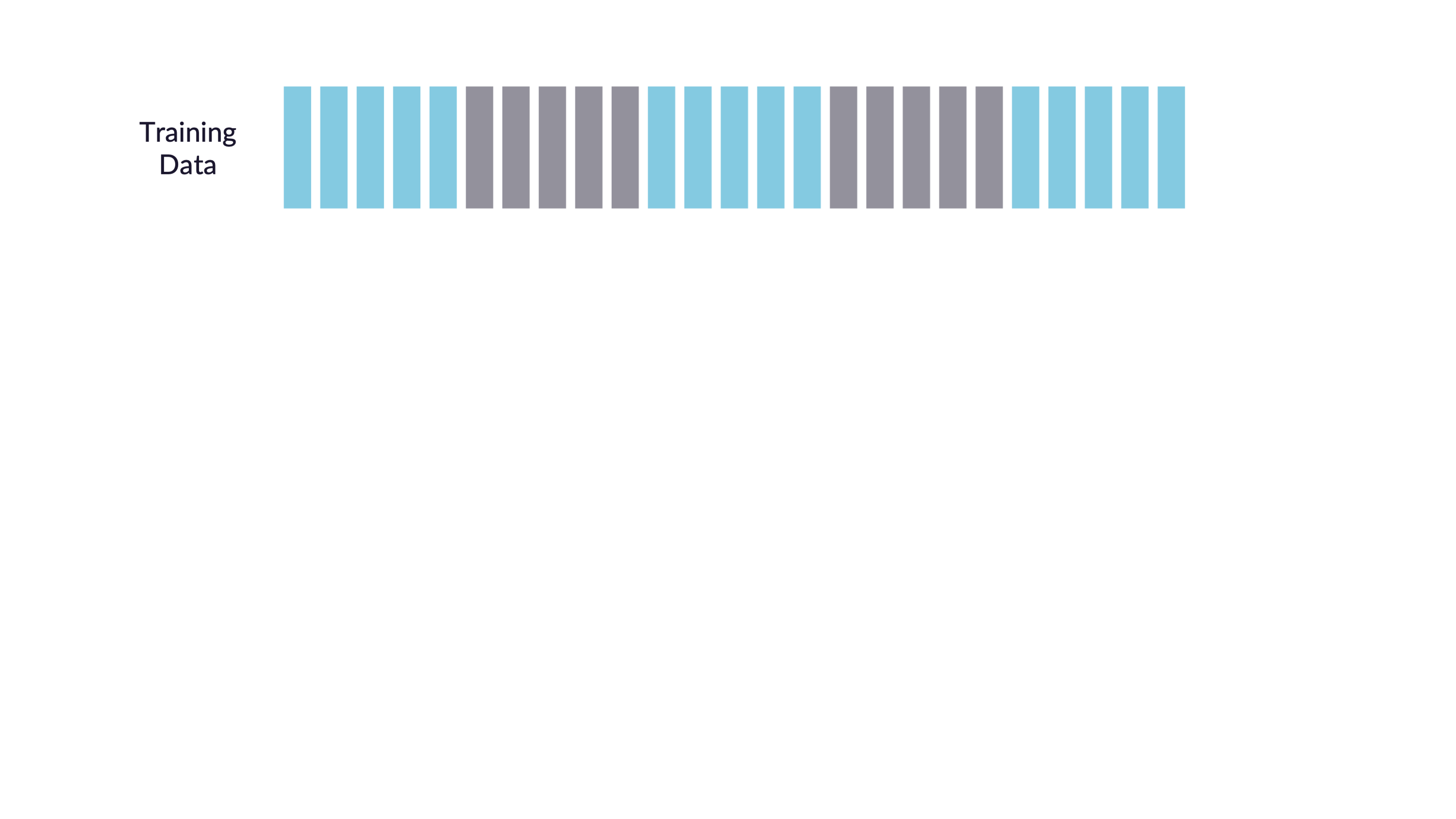
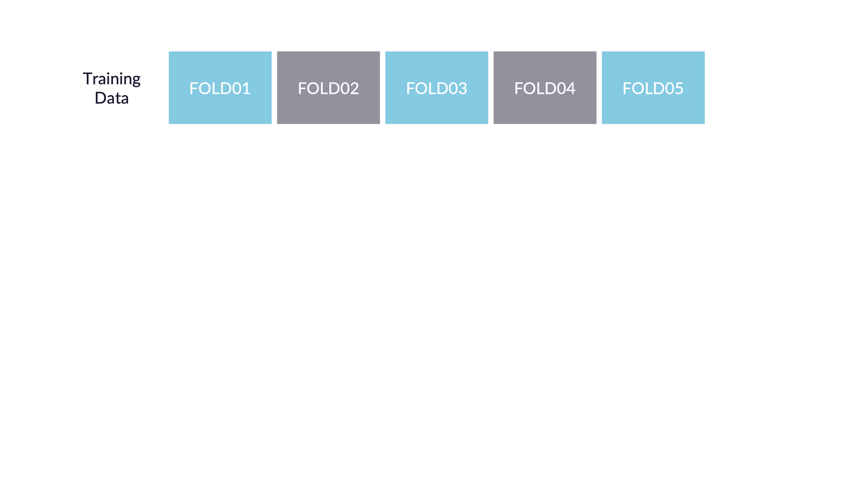
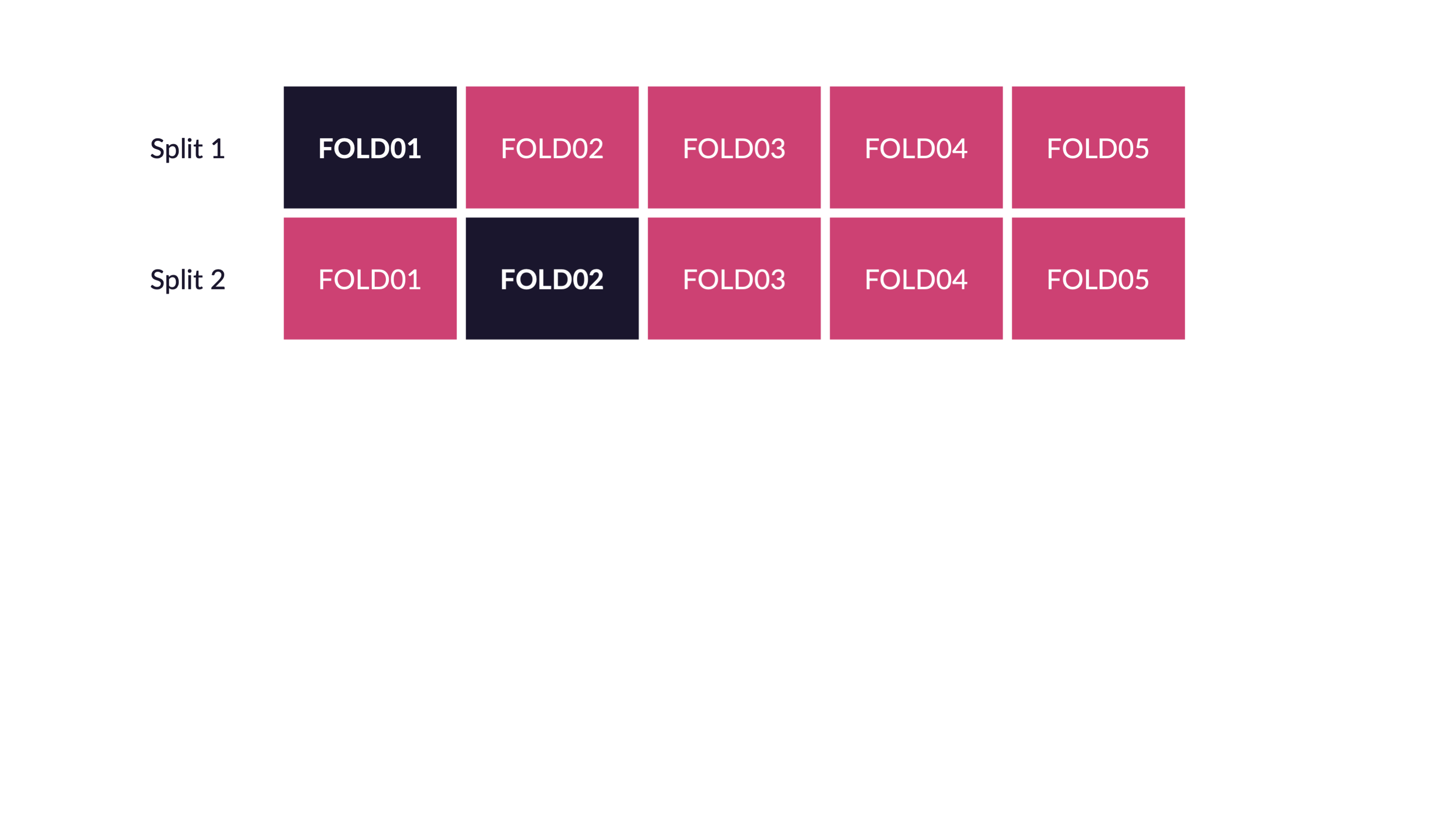
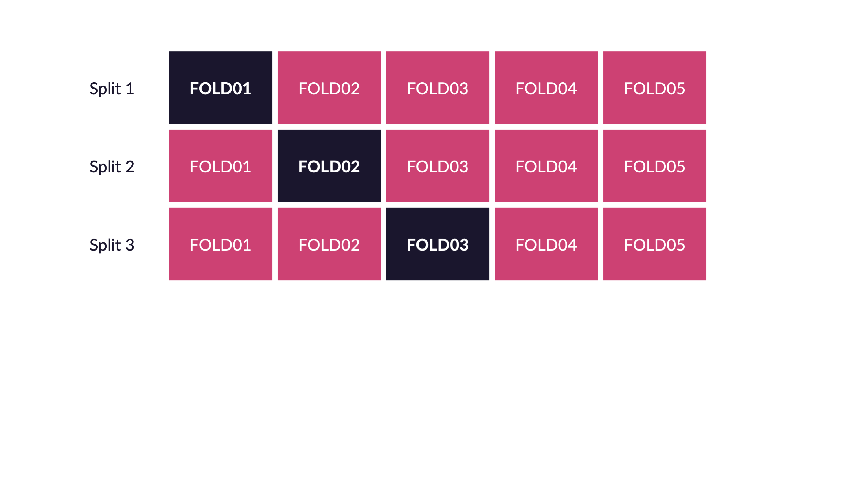
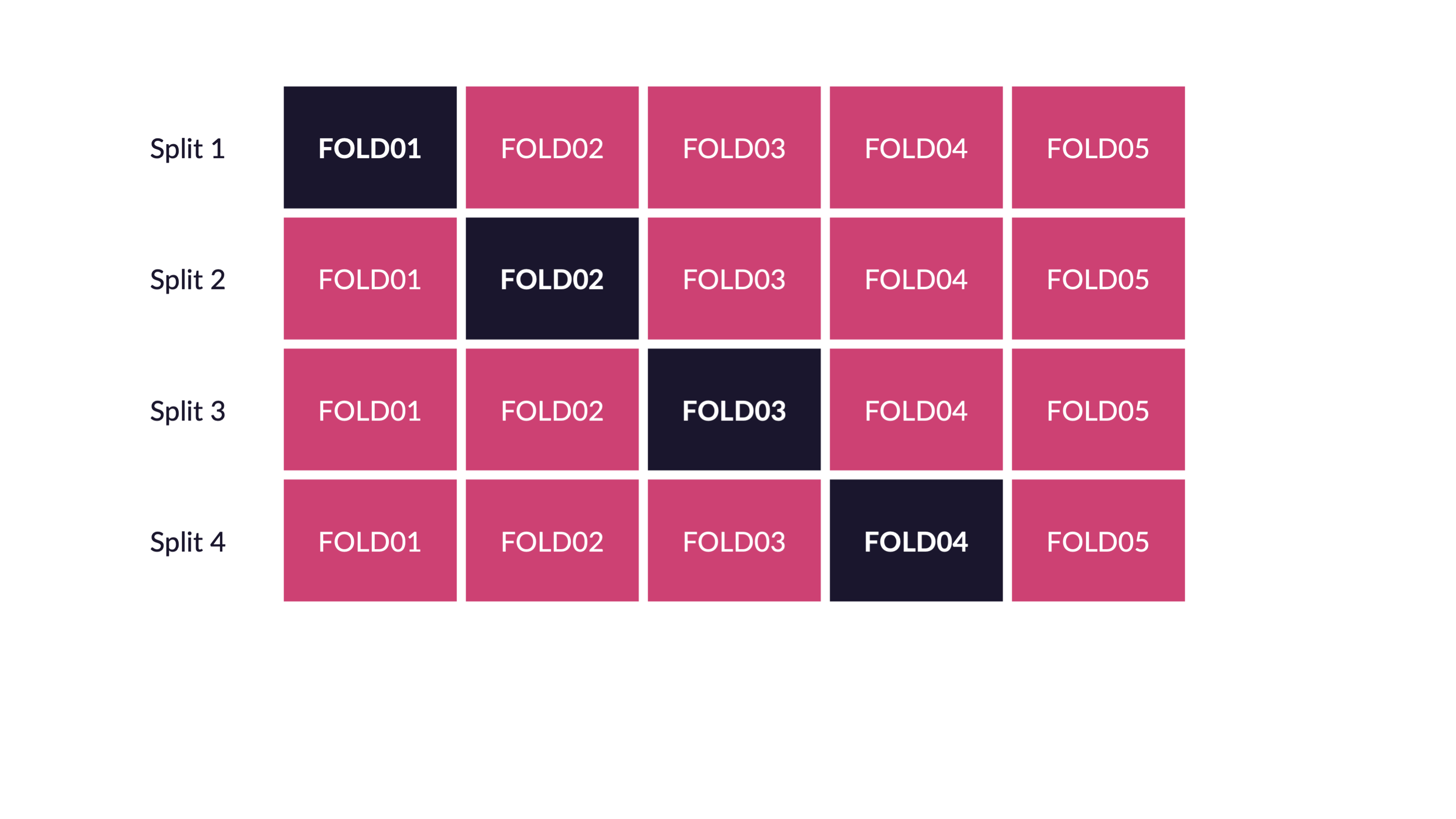
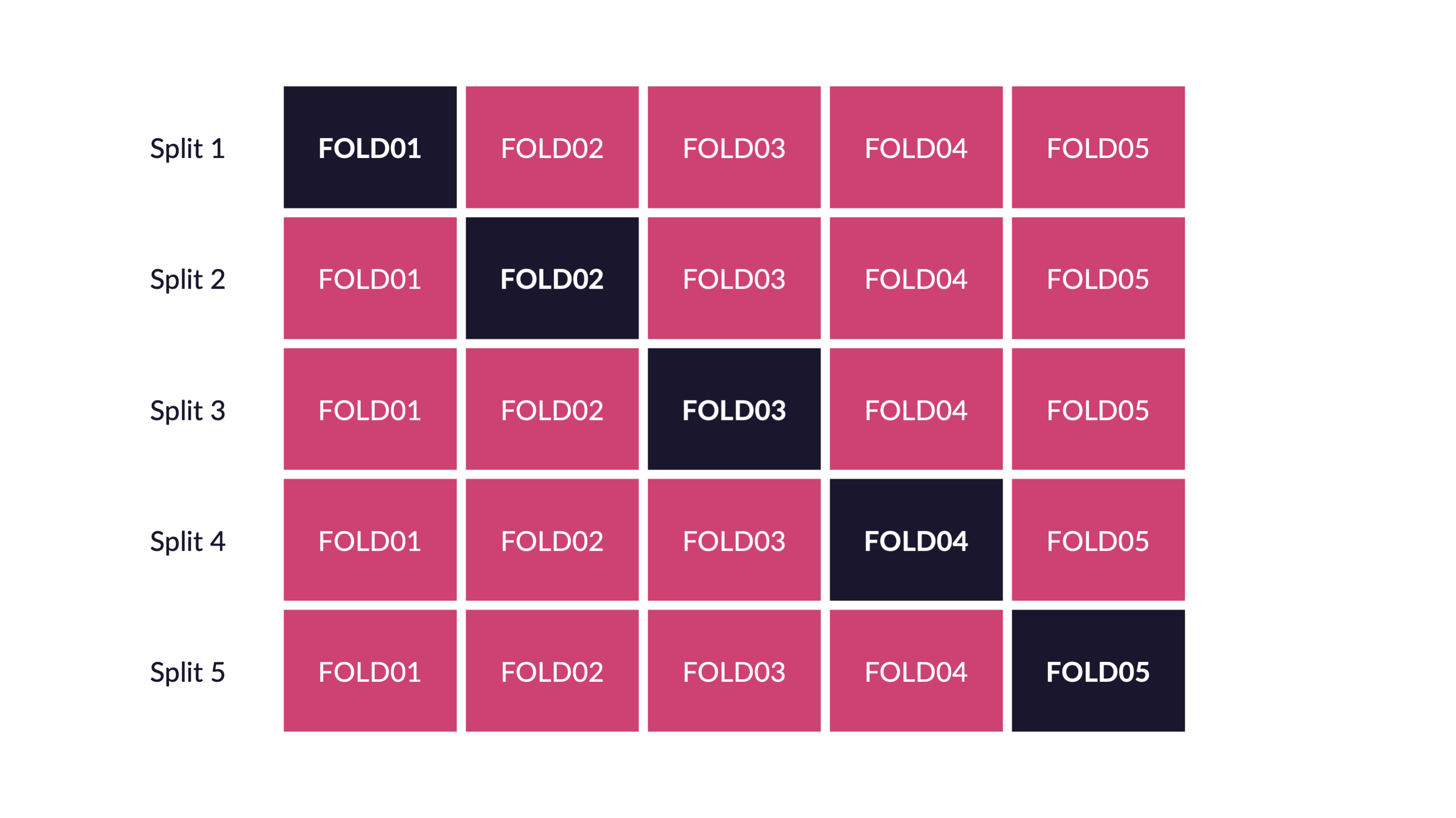
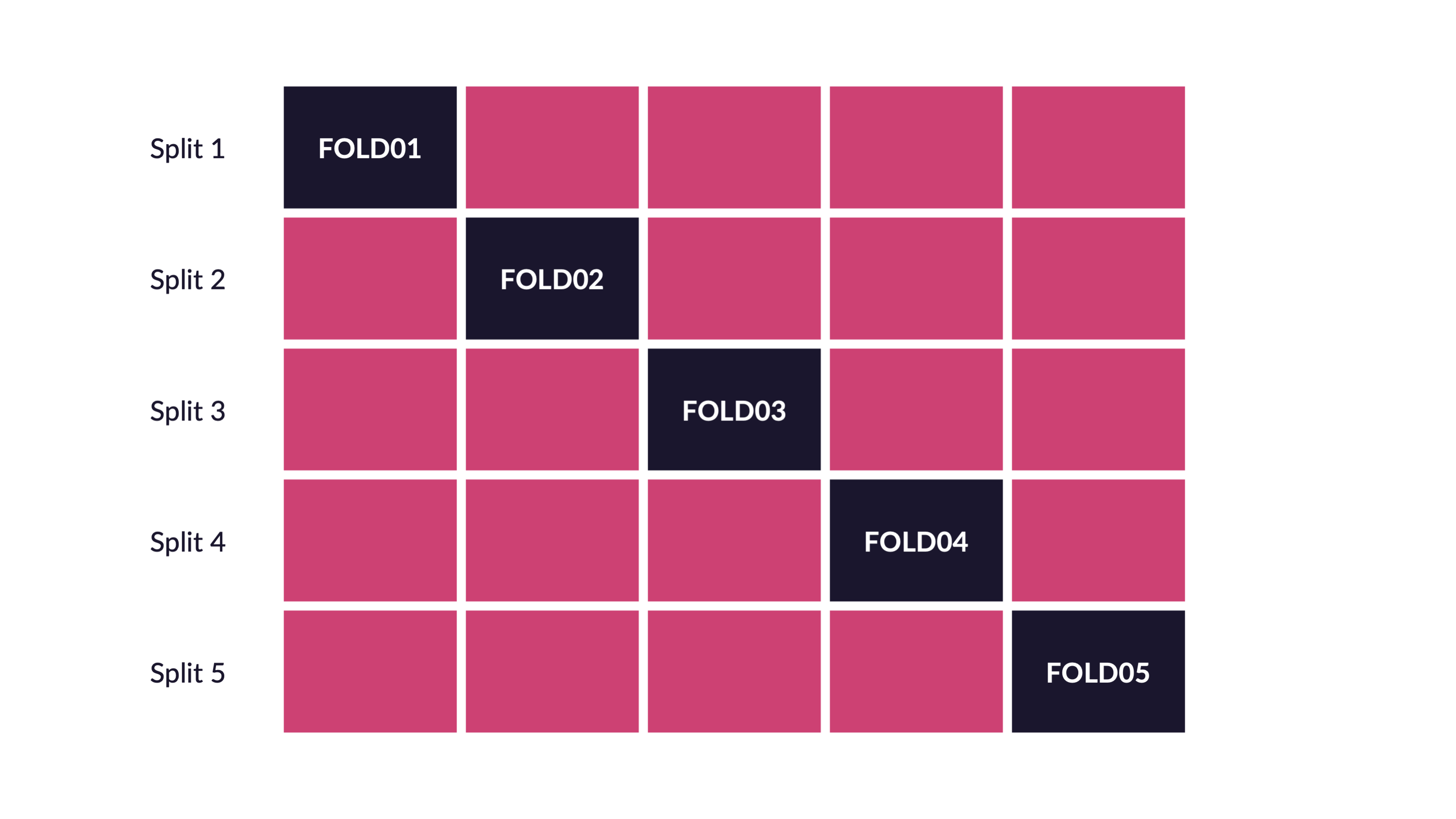
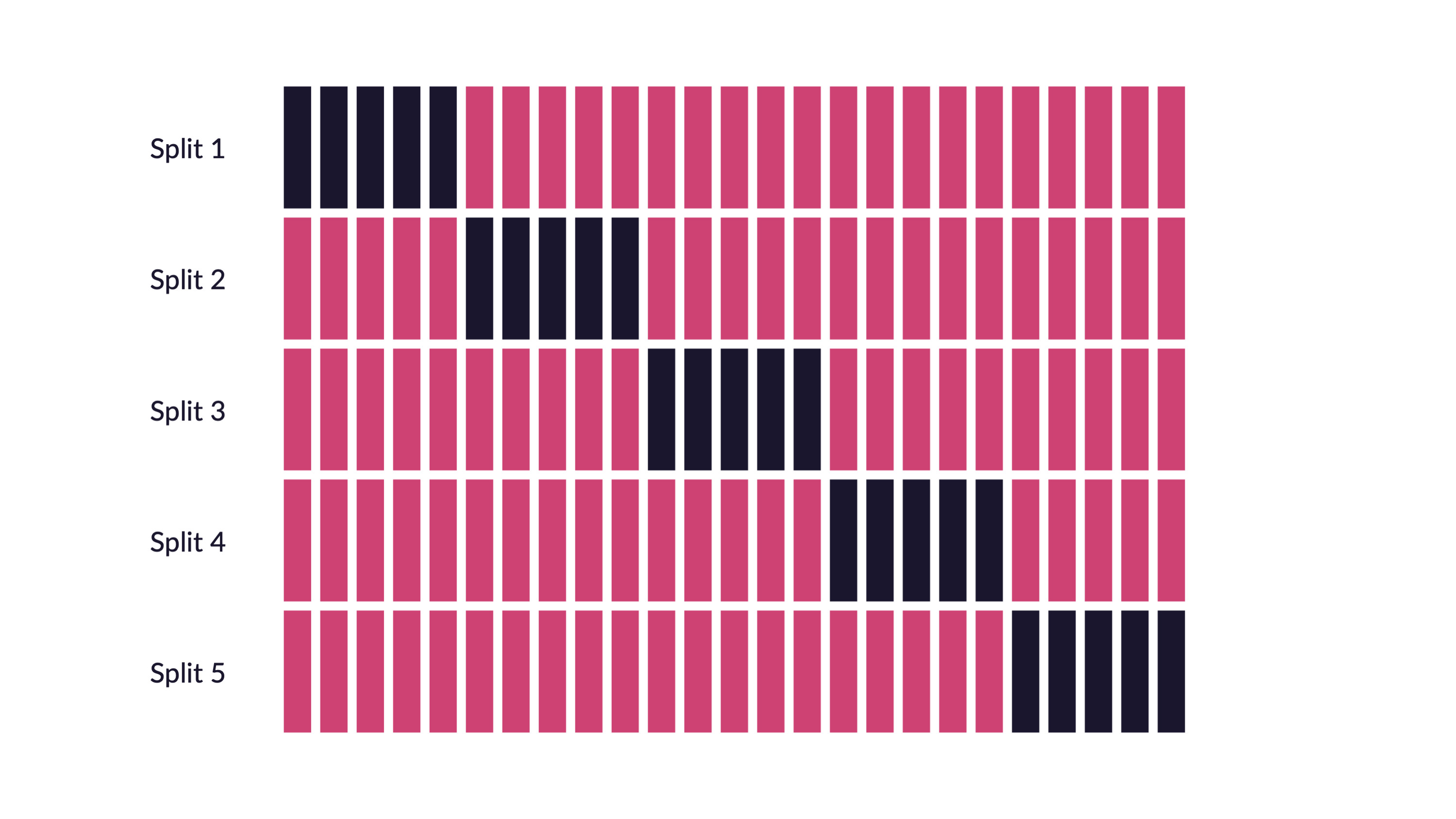
V-fold cross-validation
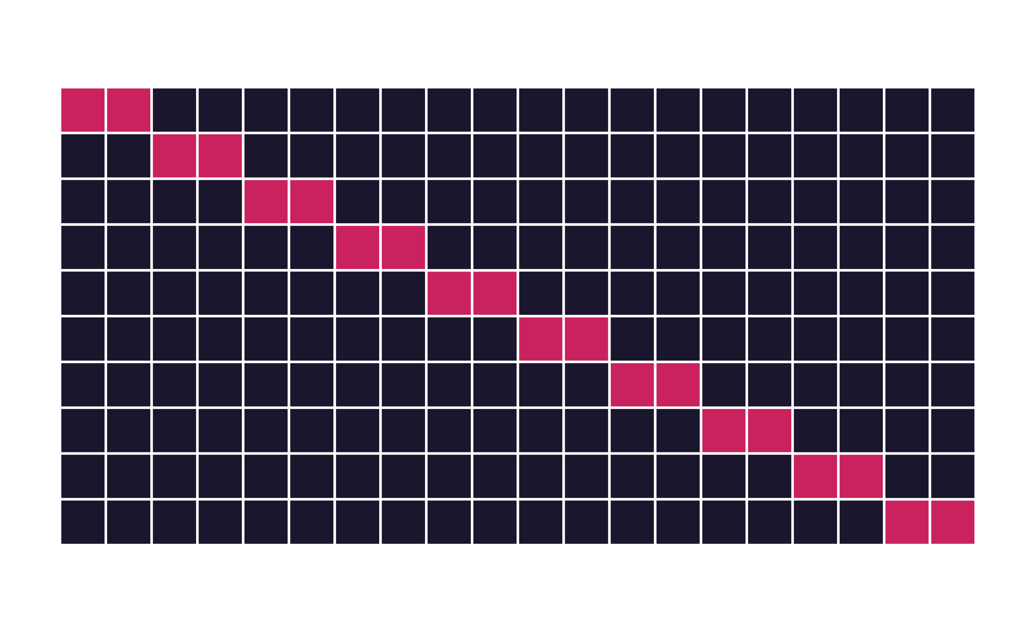
Guess
How many times does an observation/row appear in the assessment set?
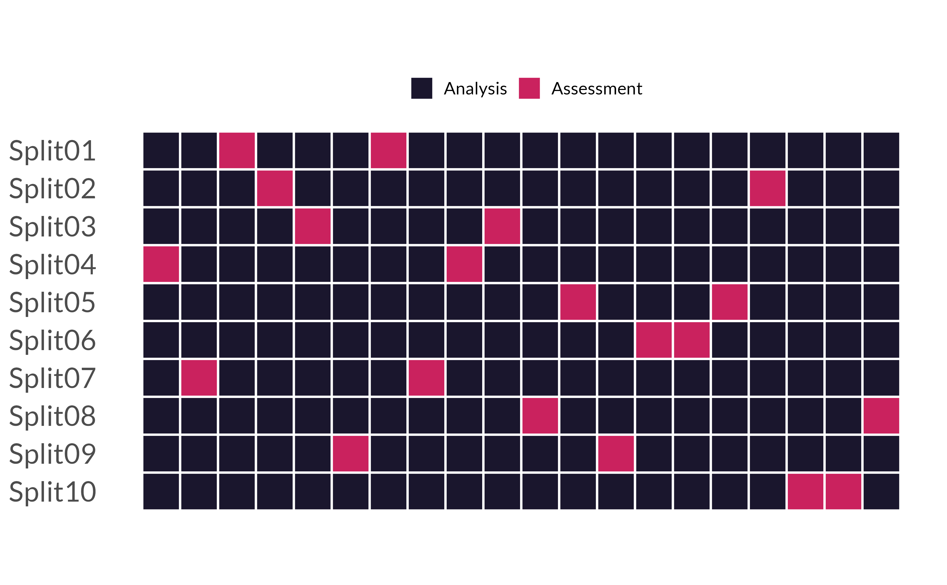
Quiz
If we use 10 folds, which percent of our data will end up in the analysis set and which percent in the assessment set for each fold?
90% - analysis
10% - assessment
⏱️ Your Turn 3
Run the code below. What does it return?
01:00
set.seed(100)
hotels_folds <- vfold_cv(data = hotels_train, v = 10)
hotels_folds
## # 10-fold cross-validation
## # A tibble: 10 × 2
## splits id
## <list> <chr>
## 1 <split [2700/300]> Fold01
## 2 <split [2700/300]> Fold02
## 3 <split [2700/300]> Fold03
## 4 <split [2700/300]> Fold04
## 5 <split [2700/300]> Fold05
## 6 <split [2700/300]> Fold06
## 7 <split [2700/300]> Fold07
## 8 <split [2700/300]> Fold08
## 9 <split [2700/300]> Fold09
## 10 <split [2700/300]> Fold10fit_resamples()
Trains and tests a resampled model.
tree_mod |>
  fit_resamples(
    children ~ average_daily_rate + stays_in_weekend_nights,
    resamples = hotels_folds
  )
## # Resampling results
## # 10-fold cross-validation
## # A tibble: 10 × 4
## splits id .metrics .notes
## <list> <chr> <list> <list>
## 1 <split [2700/300]> Fold01 <tibble [2 × 4]> <tibble>
## 2 <split [2700/300]> Fold02 <tibble [2 × 4]> <tibble>
## 3 <split [2700/300]> Fold03 <tibble [2 × 4]> <tibble>
## 4 <split [2700/300]> Fold04 <tibble [2 × 4]> <tibble>
## 5 <split [2700/300]> Fold05 <tibble [2 × 4]> <tibble>
## 6 <split [2700/300]> Fold06 <tibble [2 × 4]> <tibble>
## 7 <split [2700/300]> Fold07 <tibble [2 × 4]> <tibble>
## 8 <split [2700/300]> Fold08 <tibble [2 × 4]> <tibble>
## 9 <split [2700/300]> Fold09 <tibble [2 × 4]> <tibble>
## 10 <split [2700/300]> Fold10 <tibble [2 × 4]> <tibble>collect_metrics()
Unnest the metrics column from a tidymodels fit_resamples()
tree_fit <- tree_mod |>
  fit_resamples(
    children ~ average_daily_rate + stays_in_weekend_nights,
    resamples = hotels_folds
  )
collect_metrics(tree_fit)
## # A tibble: 2 × 6
##   .metric  .estimator  mean     n std_err .config
##   <chr>    <chr>      <dbl> <int>   <dbl> <chr>
## 1 accuracy binary     0.696    10  0.0105 Preprocessor1_Mod…
## 2 roc_auc binary 0.697 10 0.0104 Preprocessor1_Mod…collect_metrics(tree_fit, summarize = FALSE)
## # A tibble: 20 × 5
## id .metric .estimator .estimate .config
## <chr> <chr> <chr> <dbl> <chr>
## 1 Fold01 accuracy binary 0.677 Preprocessor1_Model1
## 2 Fold01 roc_auc binary 0.670 Preprocessor1_Model1
## 3 Fold02 accuracy binary 0.73 Preprocessor1_Model1
## 4 Fold02 roc_auc binary 0.731 Preprocessor1_Model1
## 5 Fold03 accuracy binary 0.683 Preprocessor1_Model1
## 6 Fold03 roc_auc binary 0.698 Preprocessor1_Model1
## 7 Fold04 accuracy binary 0.71 Preprocessor1_Model1
## 8 Fold04 roc_auc binary 0.718 Preprocessor1_Model1
## 9 Fold05 accuracy binary 0.737 Preprocessor1_Model1
## 10 Fold05 roc_auc binary 0.735 Preprocessor1_Model1
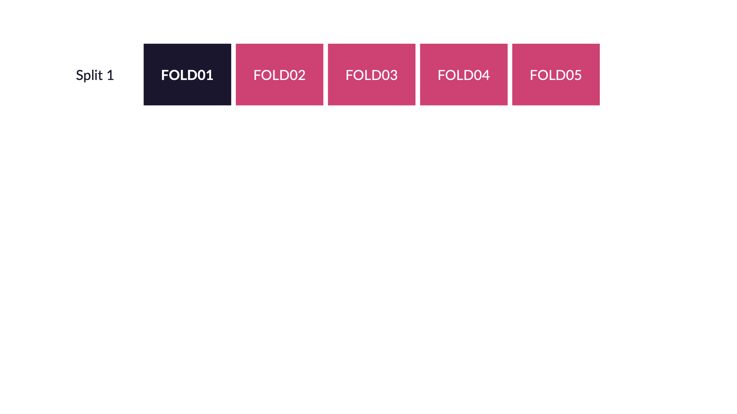
## # ℹ 10 more rows10-fold CV
10 different analysis/assessment sets
10 different models (trained on analysis sets)
10 different sets of performance statistics (on assessment sets)
📏 Evaluate models with yardstick
yardstick
https://tidymodels.github.io/yardstick/articles/metric-types.html#metrics
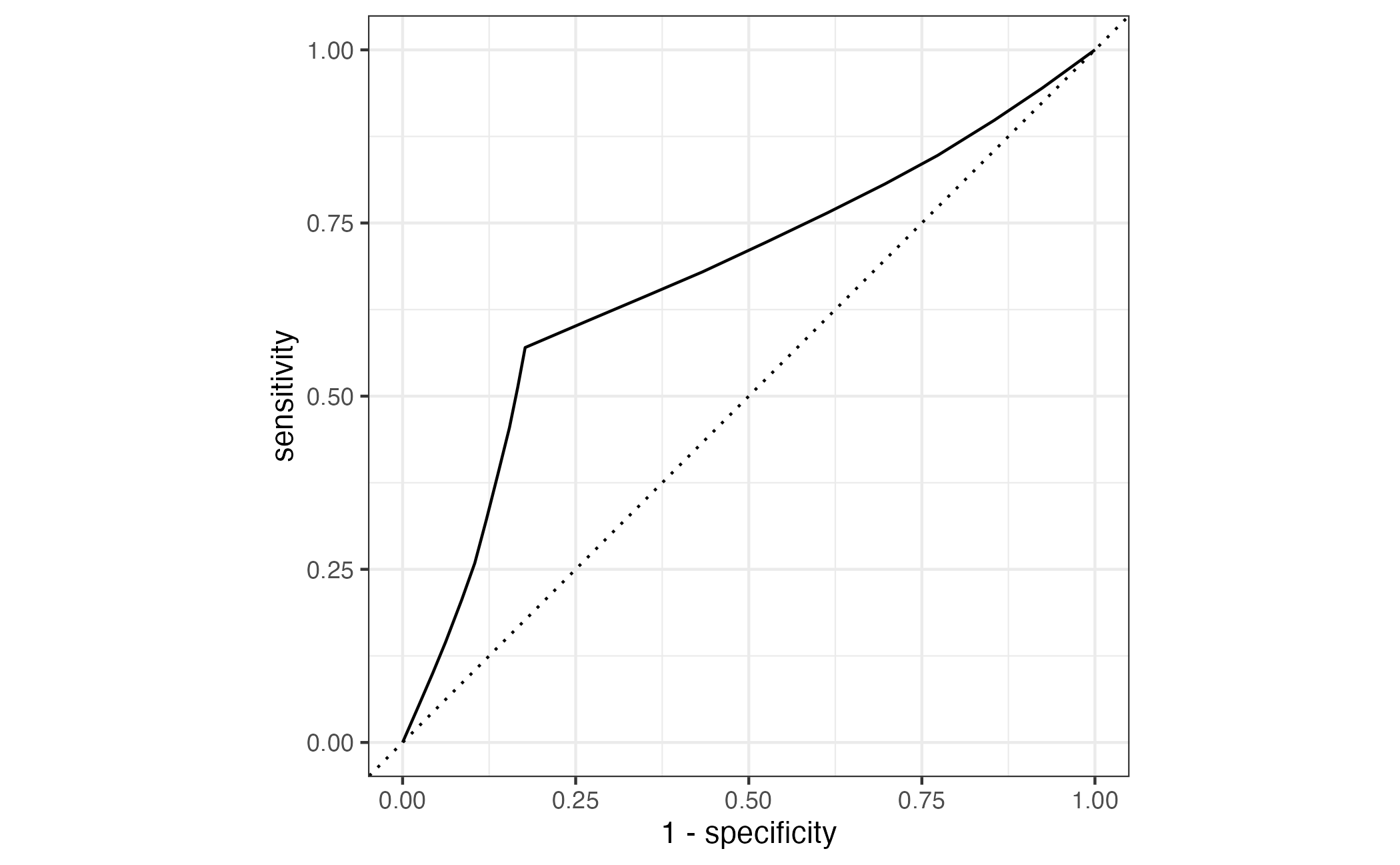
roc_curve()
Takes predictions from a special kind of fit_resamples().
Returns a tibble with probabilities.
truth = actual outcome
... = predicted probability of outcome
tree_preds <- tree_mod |>
fit_resamples(
children ~ average_daily_rate + stays_in_weekend_nights,
resamples = hotels_folds,
control = control_resamples(save_pred = TRUE)
)
tree_preds |>
collect_predictions() |>
roc_curve(truth = children, .pred_children)
## # A tibble: 22 × 3
## .threshold specificity sensitivity
## <dbl> <dbl> <dbl>
## 1 -Inf 0 1
## 2 0.335 0 1
## 3 0.338 0.0762 0.945
## 4 0.339 0.146 0.898
## 5 0.343 0.227 0.848
## 6 0.345 0.303 0.806
## 7 0.346 0.387 0.764
## 8 0.347 0.474 0.723
## 9 0.348 0.567 0.679
## 10 0.349 0.648 0.645
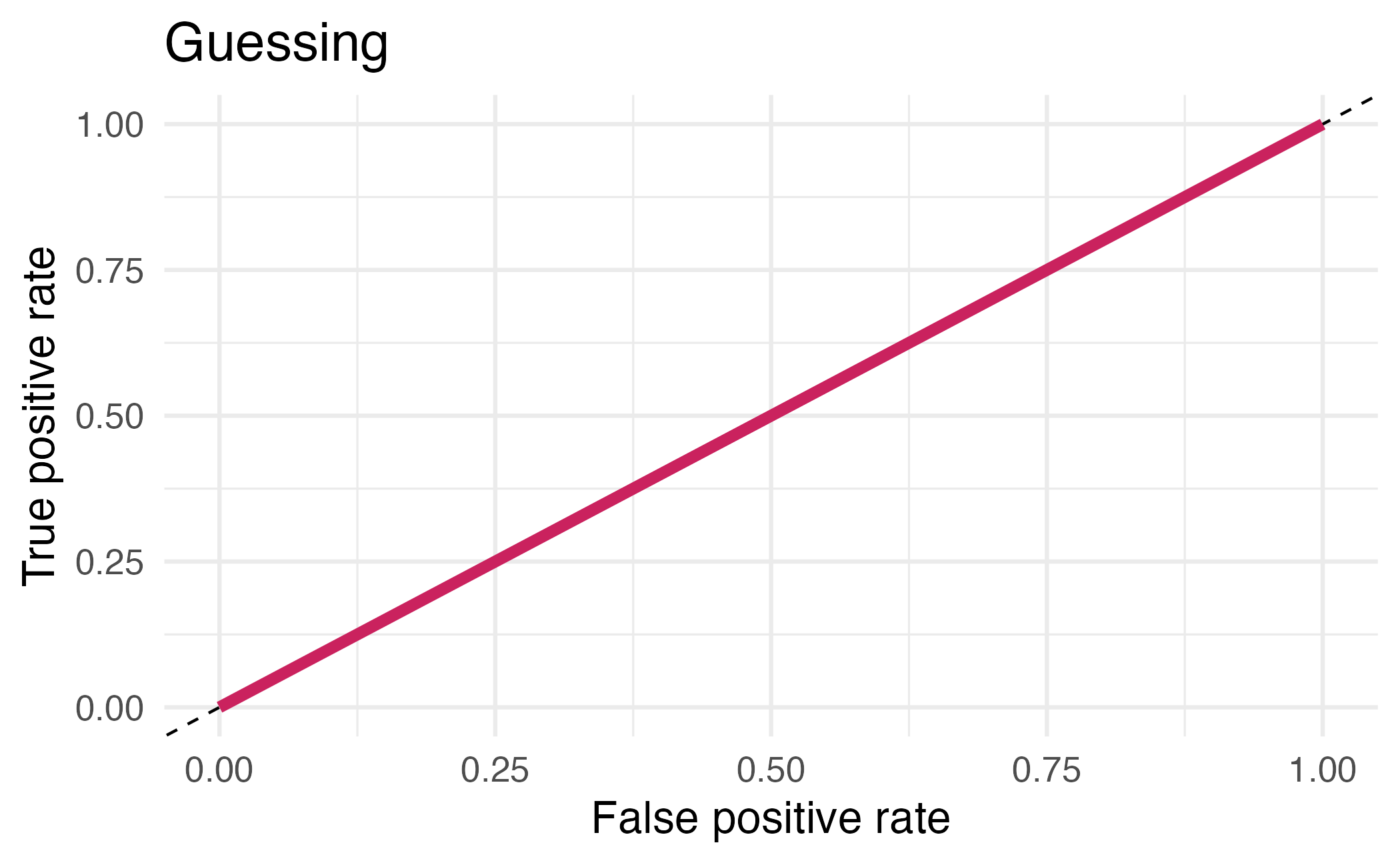
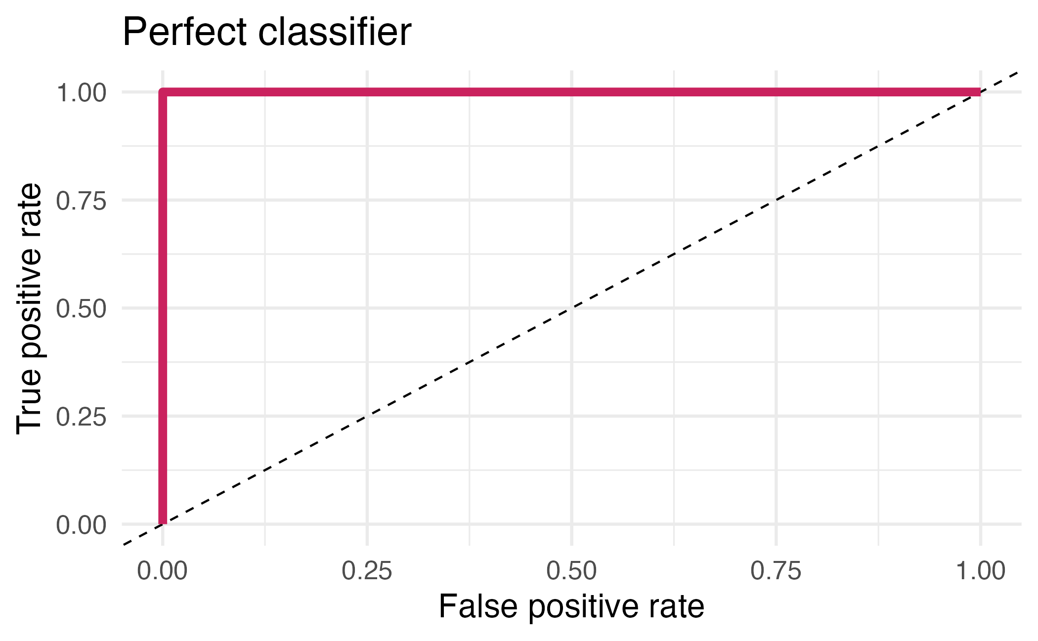
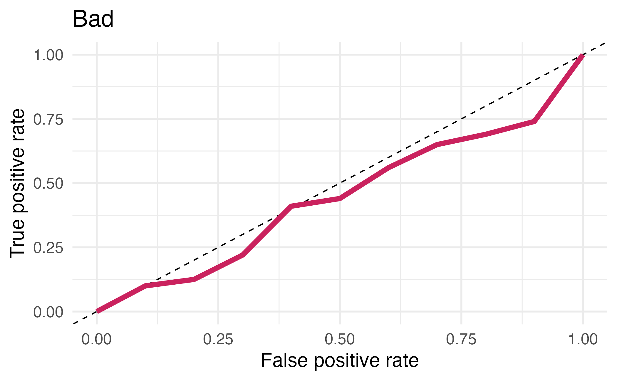
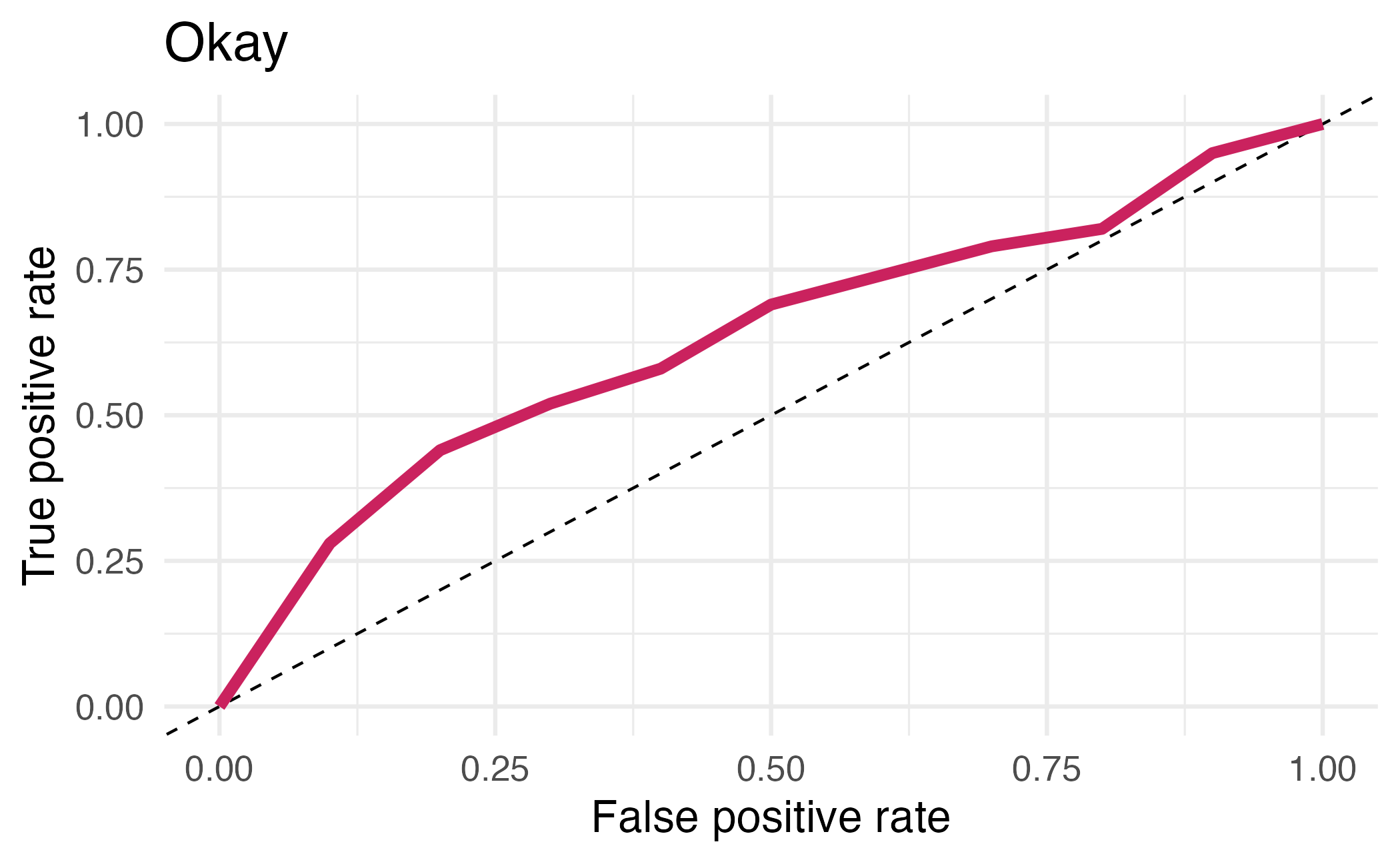
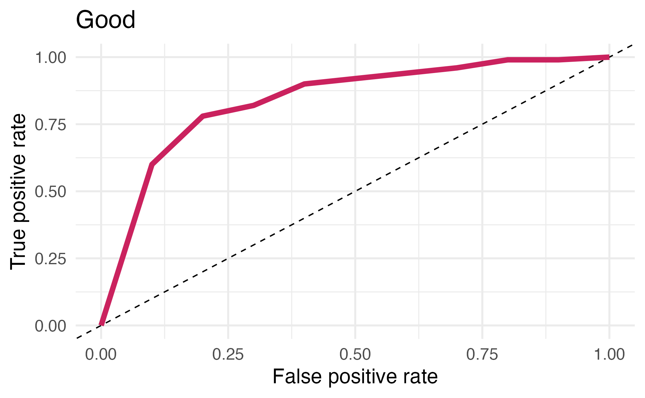
## # ℹ 12 more rowsArea under the curve
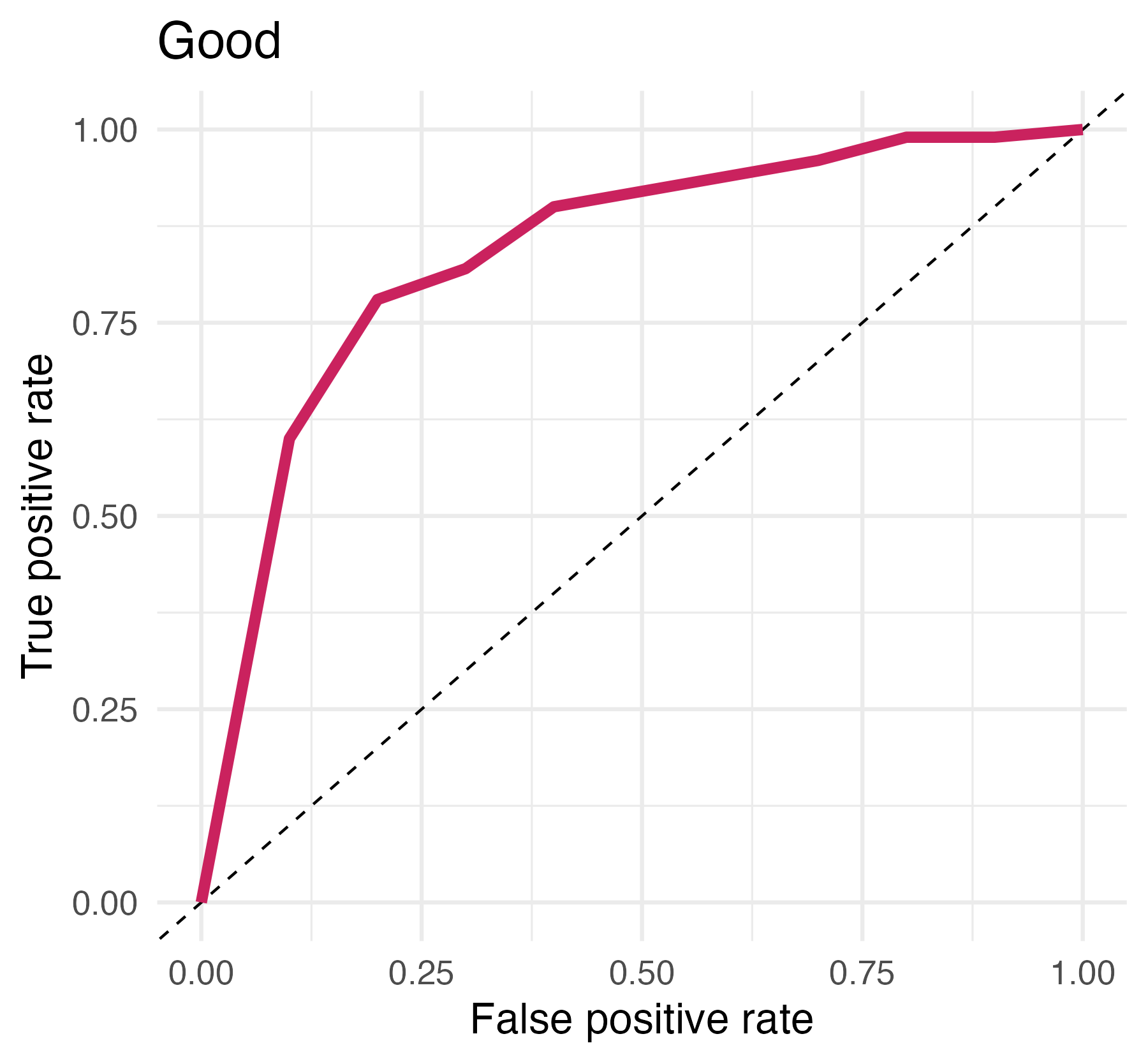
AUC = 0.5: random guessing
AUC = 1: perfect classifier
In general AUC of above 0.8 considered “good”
⏱️ Your turn 4
Add an autoplot() to visualize the ROC AUC.
Recap
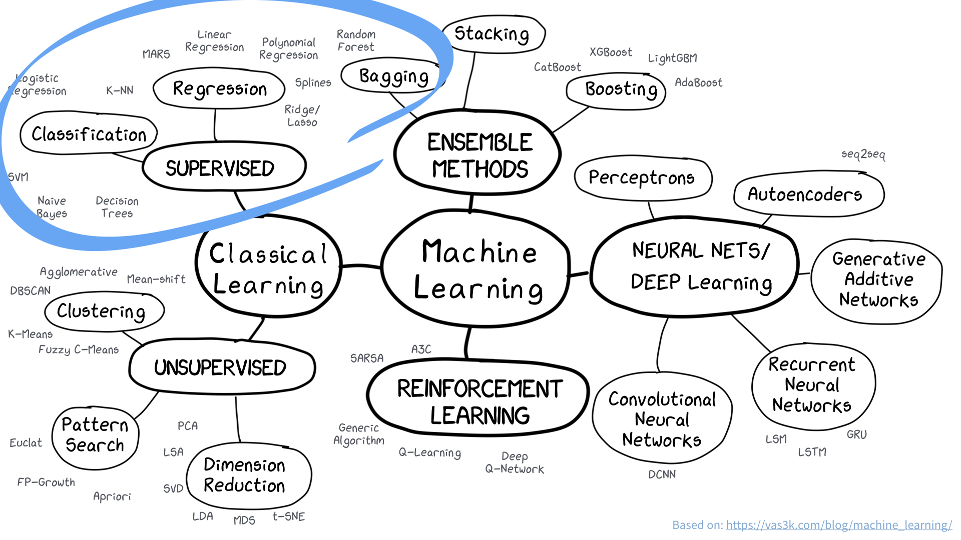
- Machine learning is an extremely vast field containing a range of methodologies
- Supervised learning is used to predict outcomes
- To avoid bias in your model, use training/testing sets and cross-validation to partition your data
- Assess model performance using appropriate metrics on the assessment sets
Acknowledgments
- Materials derived from Tidymodels, Virtually by Allison Hill and licensed under a Creative Commons Attribution-ShareAlike 4.0 International (CC BY-SA) License.
- Dataset and some modeling steps derived from A predictive modeling case study and licensed under a Creative Commons Attribution-ShareAlike 4.0 International (CC BY-SA) License.