Tree-based inference and hyperparameter optimization

Lecture 24

Dr. Benjamin Soltoff

Cornell University
INFO 2950 - Spring 2024

April 23, 2024

Announcements

Project drafts
Working as a team
Appropriate use of generative AI

Application exercise

`ae-22`

Go to the course GitHub org and find your ae-22 (repo name will be suffixed with your GitHub name).
Clone the repo in RStudio Workbench, open the Quarto document in the repo, and follow along and complete the exercises.
Render, commit, and push your edits by the AE deadline – end of tomorrow

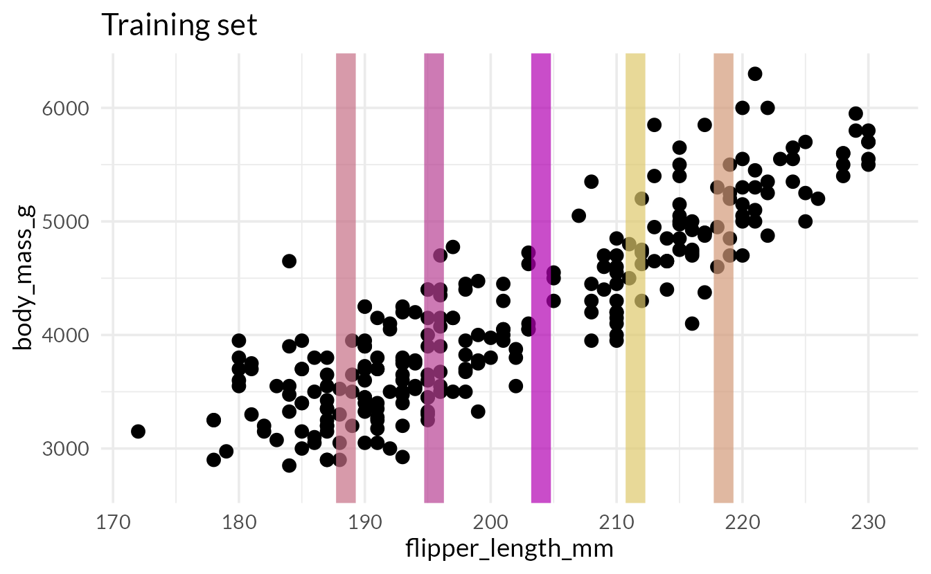
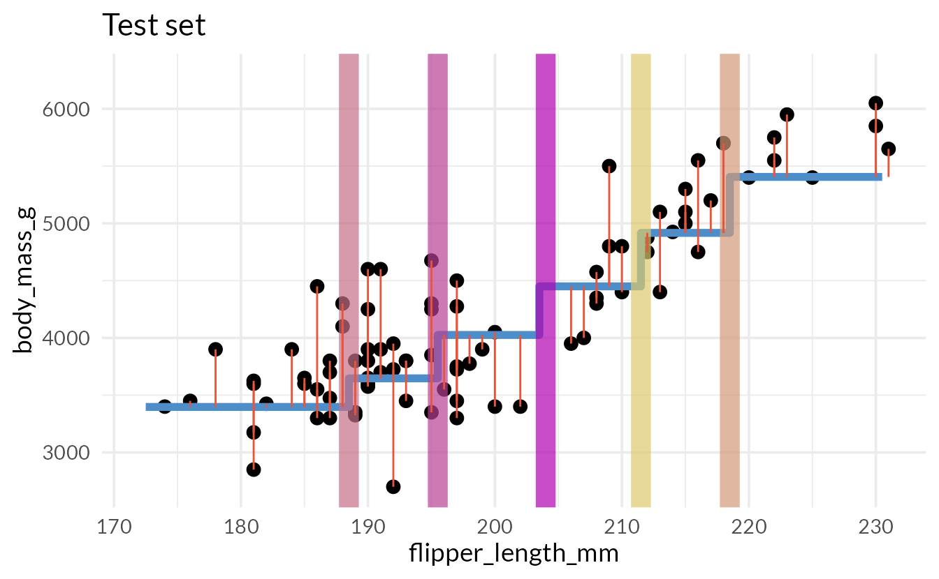
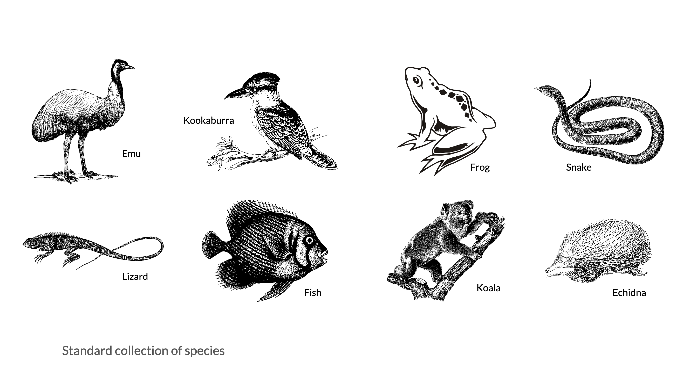
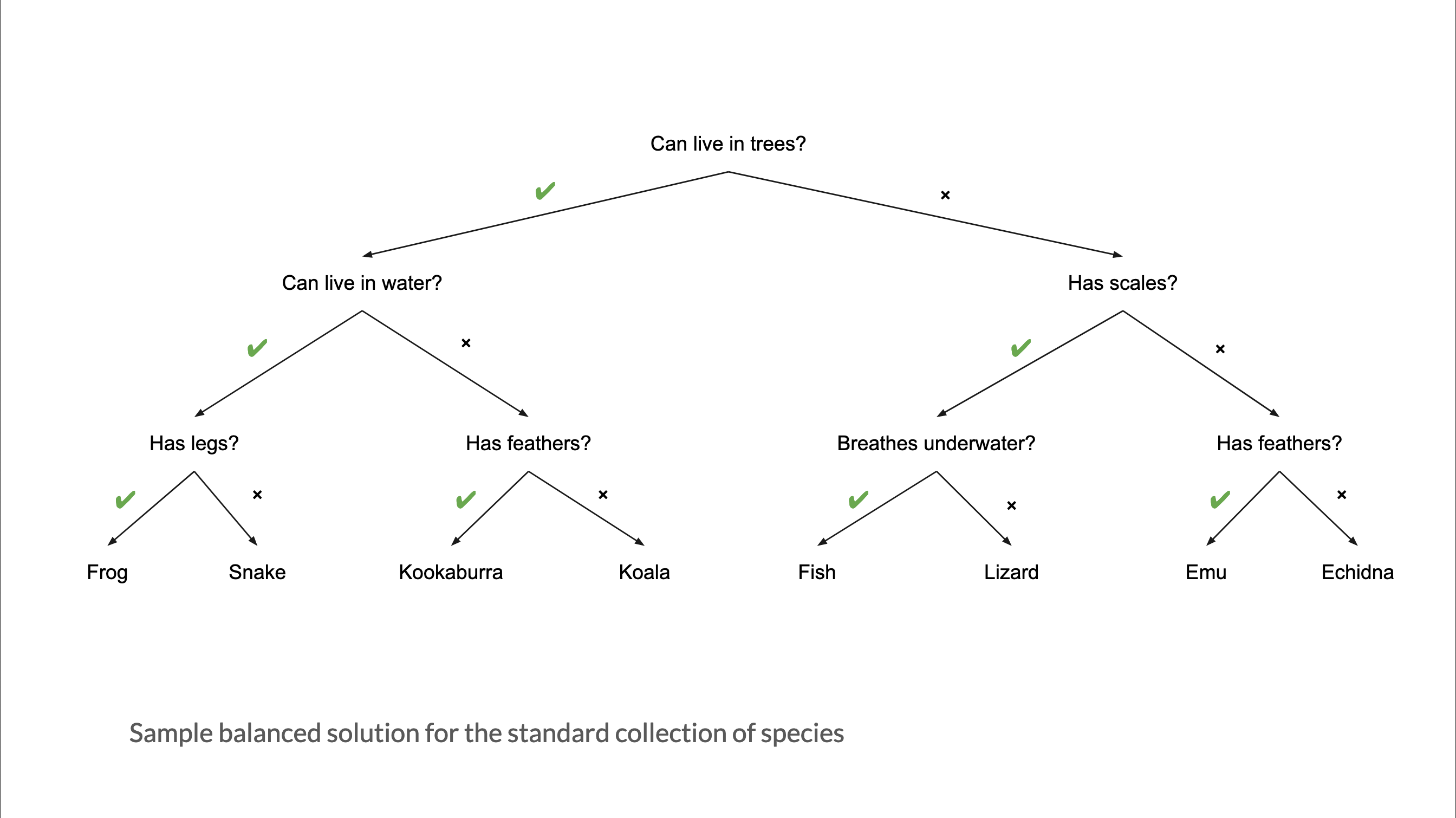
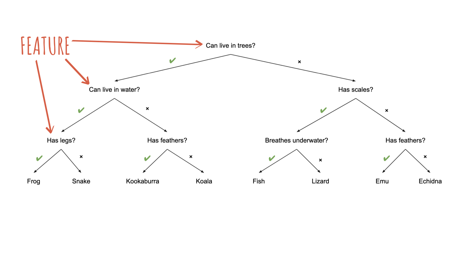
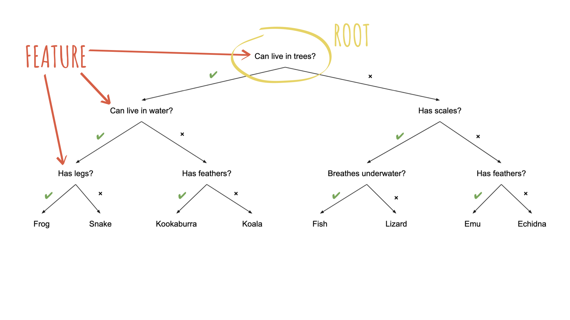
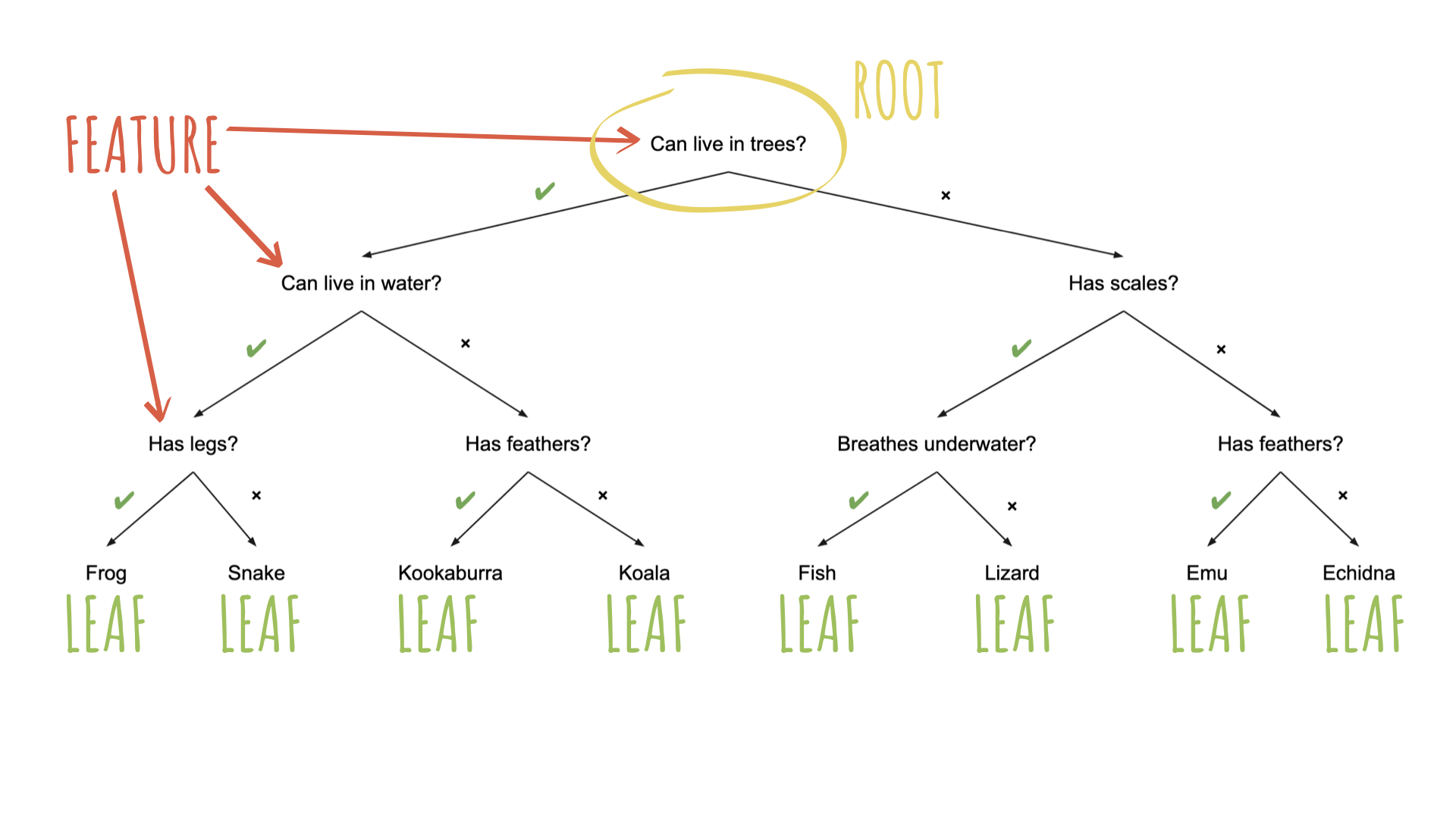
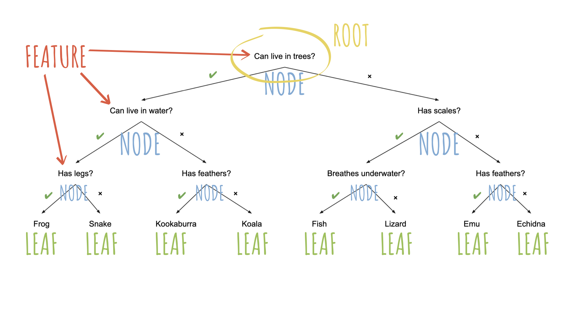
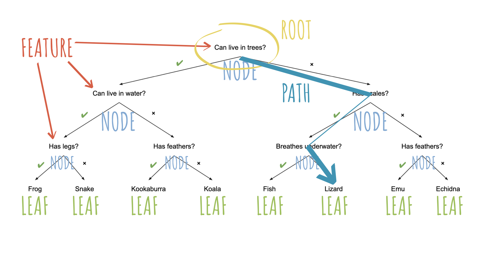
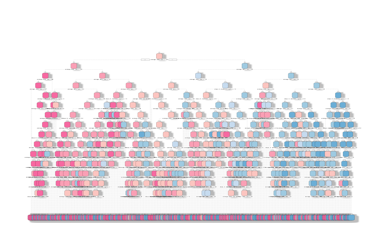
Decision trees

Decision Trees

To predict the outcome of a new data point:

Uses rules learned from splits
Each split maximizes information gain

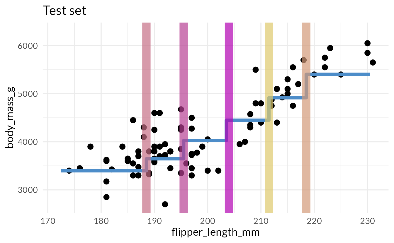
Quiz

How do we assess predictions here?

Root Mean Squared Error (RMSE)

Uses of decision trees

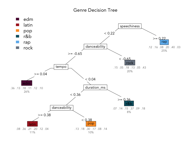
What makes a good guesser?

High information gain per question (can it fly?)

Clear features (feathers vs. is it “small”?)

Order of features matters

To specify a model with `parsnip`

1. Pick a model + engine

2. Set the mode (if needed)

To specify a decision tree model with `parsnip`

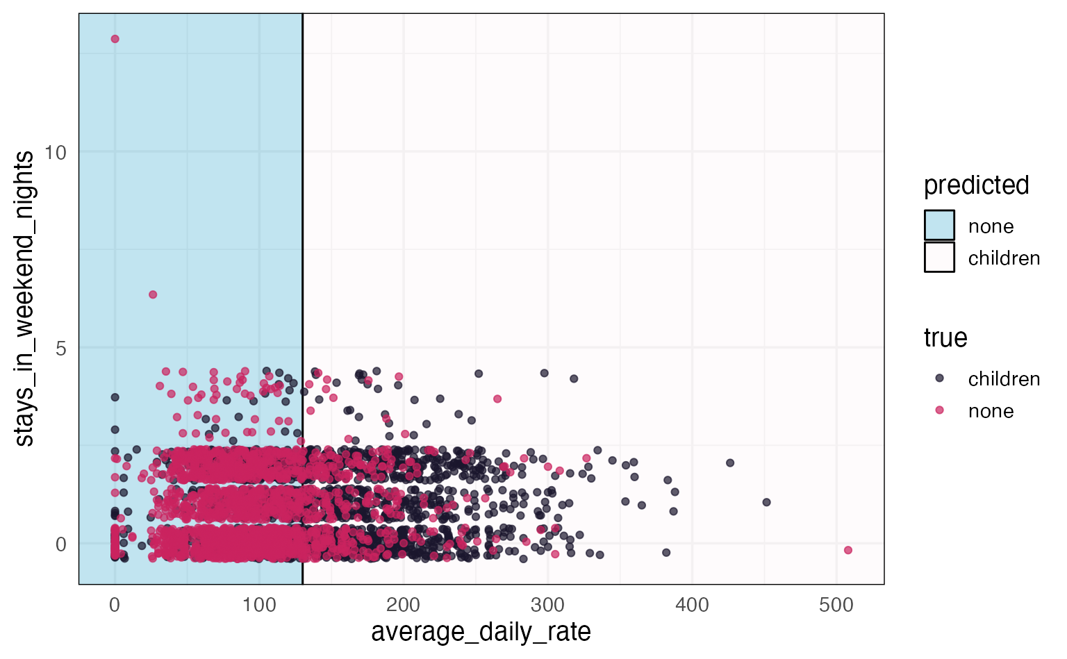
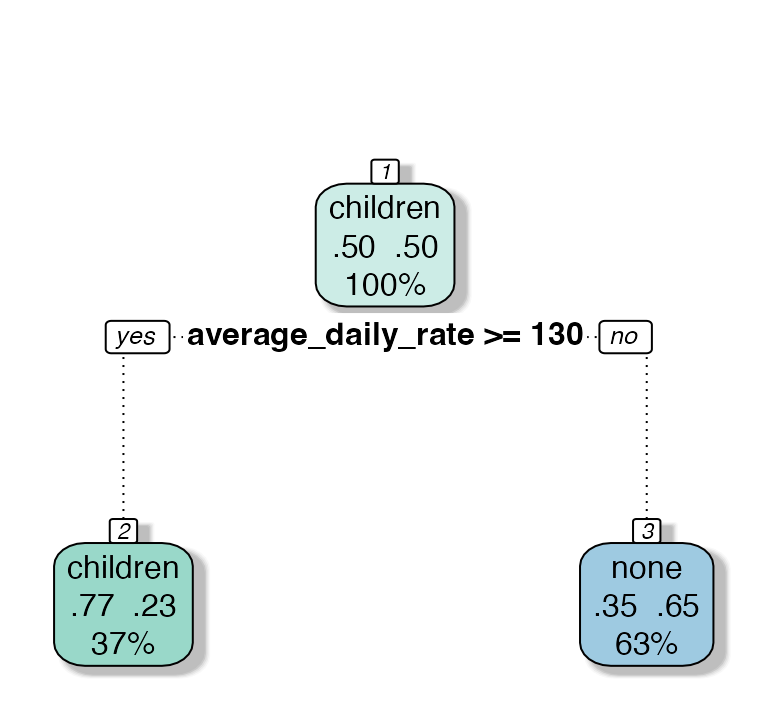
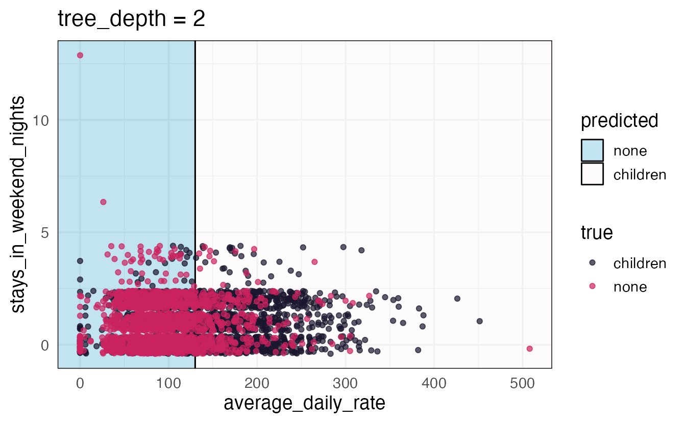
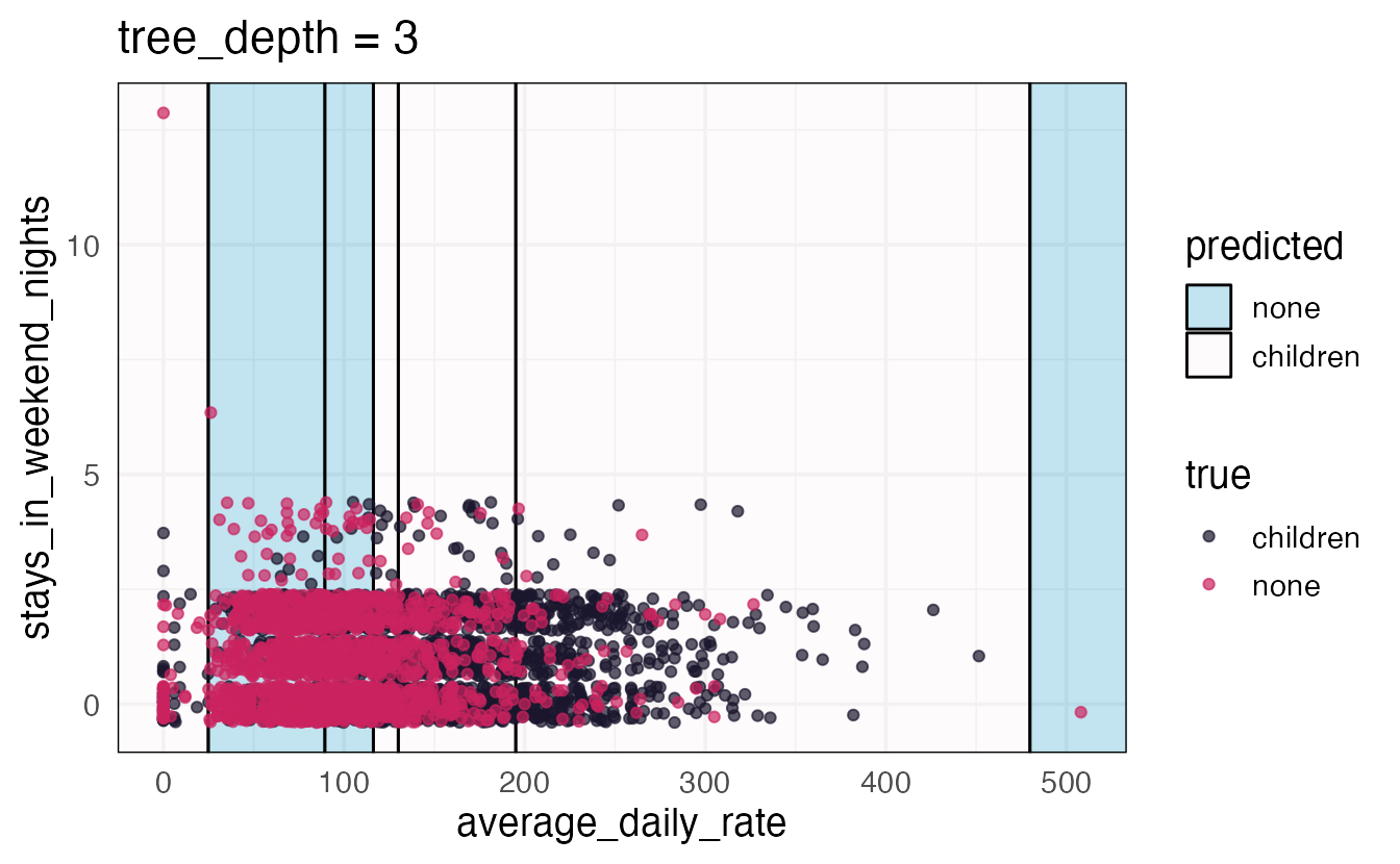
tree_mod <- decision_tree(engine = "rpart") |>
  set_mode("classification")

 nn children  chi non                                   cover
  2 children [.77 .23] when average_daily_rate >= 130     37%
  3     none [.35 .65] when average_daily_rate <  130     63%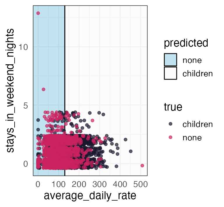

⏱️ Your turn 1

Here is our very-vanilla parsnip model specification for a decision tree (also in your qmd)…

tree_mod <- decision_tree(engine = "rpart") |>
  set_mode("classification")

And a workflow:

tree_wf <- workflow() |>
  add_formula(children ~ .) |>
  add_model(tree_mod)

For decision trees, no recipe really required 🎉

⏱️ Your turn 1

Fill in the blanks to return the accuracy and ROC AUC for this model using 10-fold cross-validation.

02:00

set.seed(100)
tree_wf |>
  fit_resamples(resamples = hotels_folds) |>
  collect_metrics()

# A tibble: 3 × 6
  .metric     .estimator  mean     n std_err .config        
  <chr>       <chr>      <dbl> <int>   <dbl> <chr>          
1 accuracy    binary     0.786    10 0.00706 Preprocessor1_…
2 brier_class binary     0.156    10 0.00417 Preprocessor1_…
3 roc_auc     binary     0.833    10 0.00840 Preprocessor1_…

Model arguments

`args()`

Print the arguments (hyperparameters) for a parsnip model specification.

args(decision_tree)

function (mode = "unknown", engine = "rpart", cost_complexity = NULL, 
    tree_depth = NULL, min_n = NULL) 
NULL

`decision_tree()`

Specifies a decision tree model

decision_tree(engine = "rpart", tree_depth = 30, min_n = 20, cost_complexity = .01)

either mode works!

`decision_tree()`

Specifies a decision tree model

decision_tree(
  engine = "rpart", # default computational engine
  tree_depth = 30, # max tree depth
  min_n = 20, # smallest node allowed
  cost_complexity = .01 # 0 > cp > 0.1
)

`set_args()`

Change the arguments for a parsnip model specification.

_mod |> set_args(tree_depth = 3)

decision_tree(engine = "rpart") |>
  set_mode("classification") |>
  set_args(tree_depth = 3)

Decision Tree Model Specification (classification)

Main Arguments:
  tree_depth = 3

Computational engine: rpart

decision_tree(engine = "rpart", tree_depth = 3) |>
  set_mode("classification")

Decision Tree Model Specification (classification)

Main Arguments:
  tree_depth = 3

Computational engine: rpart

`tree_depth`

Cap the maximum tree depth.

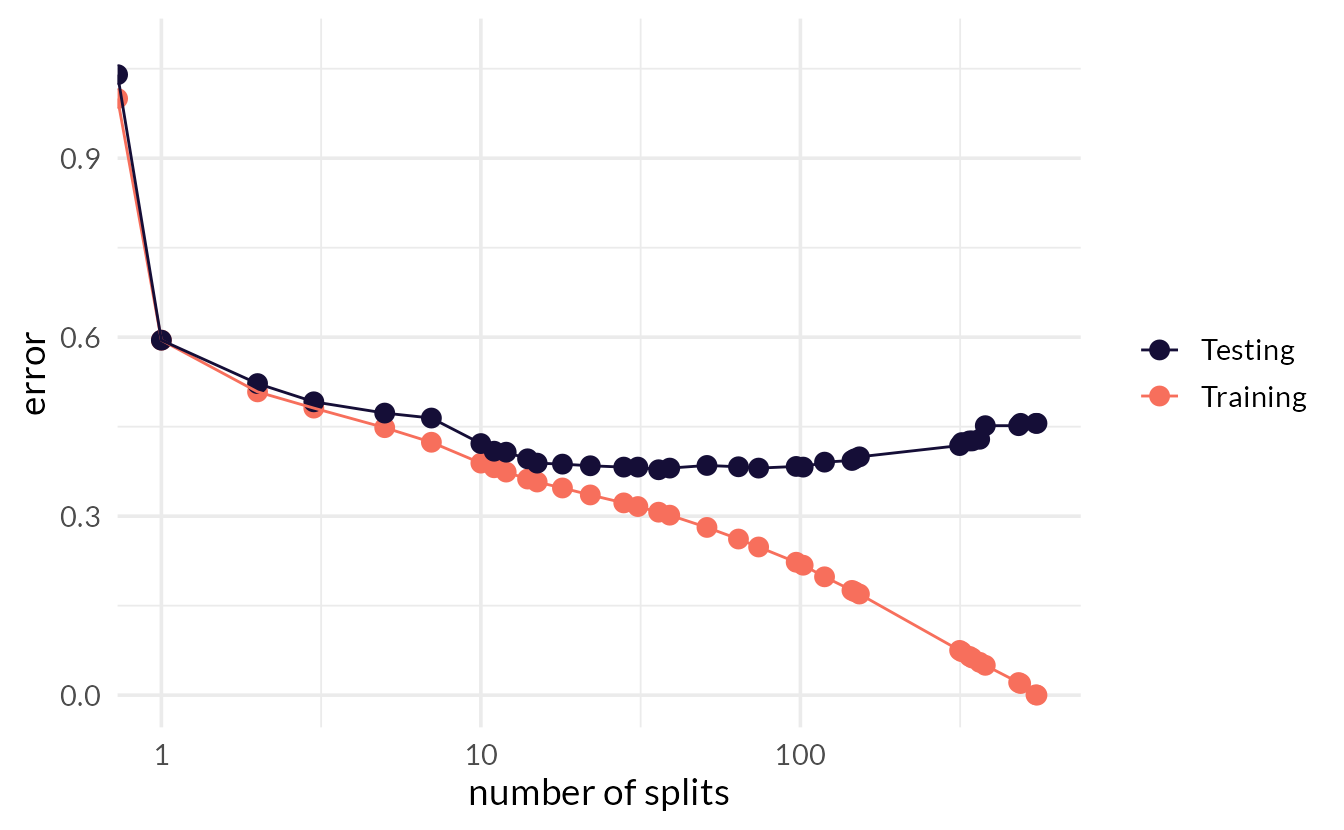
A method to stop the tree early. Used to prevent overfitting.

tree_mod |> set_args(tree_depth = 30)

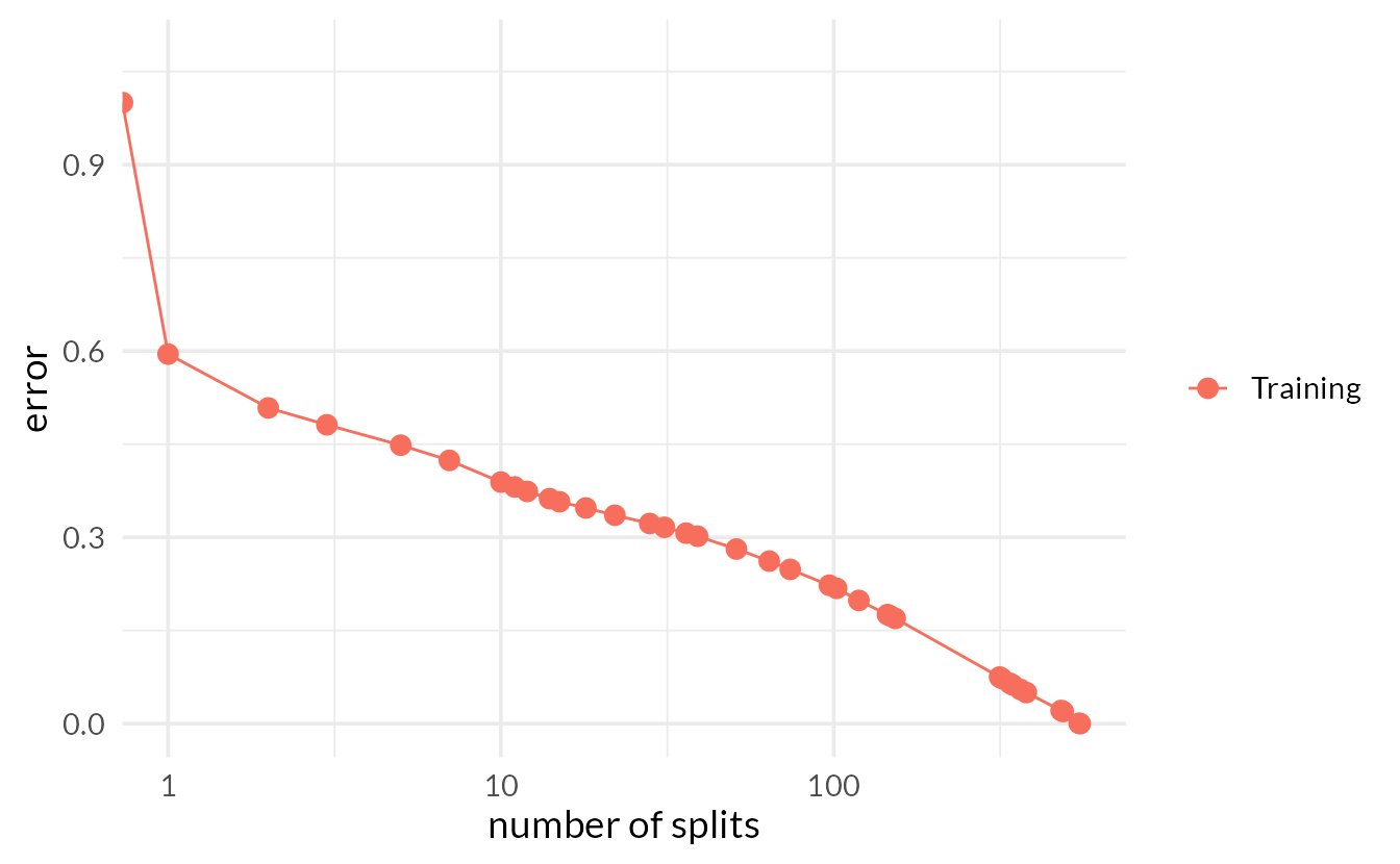
`min_n`

Set minimum n to split at any node.

Another early stopping method. Used to prevent overfitting.

tree_mod |> set_args(min_n = 20)

Quiz

What value of min_n would lead to the most overfit tree?

min_n = 1

Recap: early stopping

`parsnip` arg	`rpart` arg	default	overfit?
`tree_depth`	`maxdepth`	30	⬆️
`min_n`	`minsplit`	20	⬇️

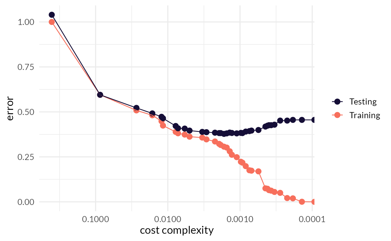
`cost_complexity`

Adds a cost or penalty to error rates of more complex trees.

A way to prune a tree. Used to prevent overfitting.

tree_mod |> set_args(cost_complexity = .01)

Closer to zero ➡️ larger trees.

Higher penalty ➡️ smaller trees.

Consider the bonsai

Small pot
Strong shears

Consider the bonsai

~~Small pot~~ Early stopping
~~Strong shears~~ Pruning

Recap: early stopping & pruning

`parsnip` arg	`rpart` arg	default	overfit?
`tree_depth`	`maxdepth`	30	⬆️
`min_n`	`minsplit`	20	⬇️
`cost_complexity`	`cp`	.01	⬇️

Axiom

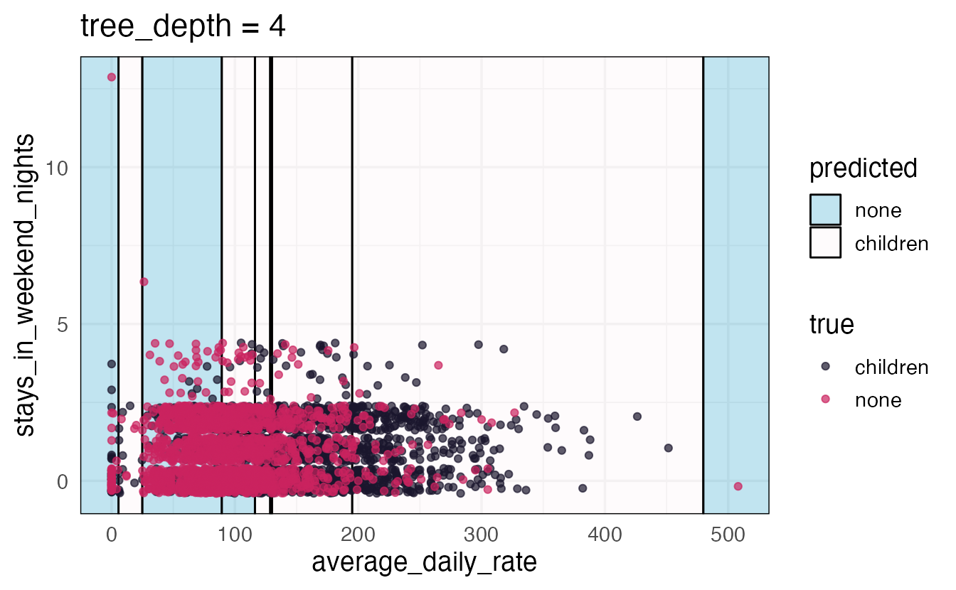
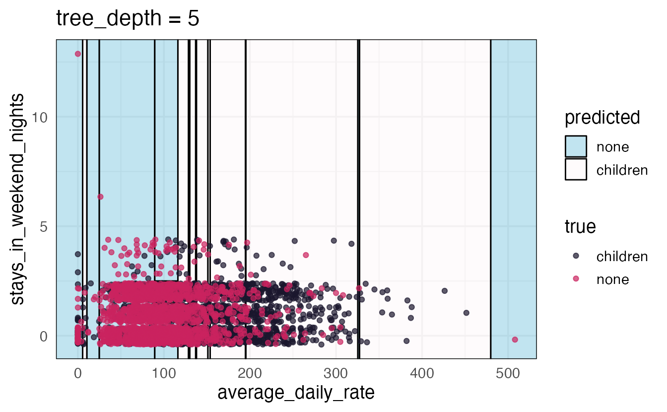
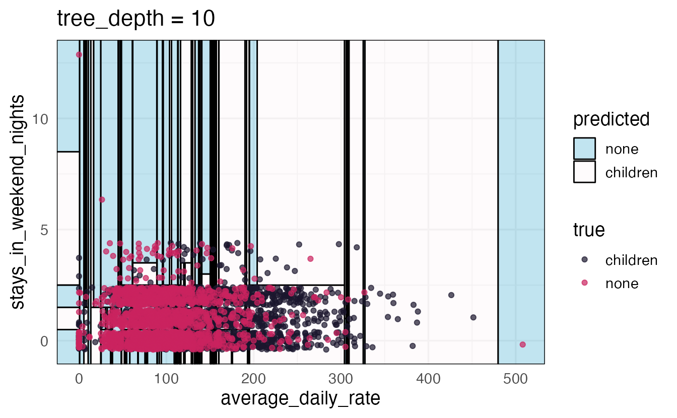
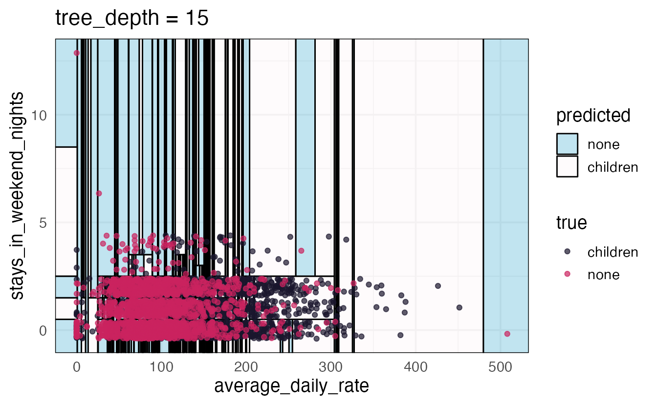
There is an inverse relationship between model accuracy and model interpretability.

Random forests

Ensemble methods

Ensemble methods combine many simple “building block” models in order to obtain a single and potentially very powerful model.¹

Individual models are typically weak learners - low accuracy on their own
Combining a set of weak learners can create a strong learner with high accuracy by reducing bias and variance

Bagging

Decision trees suffer from high variance - small changes in the data can lead to very different trees

Bootstrap aggregation (or bagging) reduces the variance of a model by averaging the predictions of many models trained on different samples of the data.

Random forests

To further improve performance over bagged trees, random forests introduce additional randomness in the model-building process to reduce the correlation across the trees.

Random feature selection: At each split, only a random subset of features are considered
Makes each individual model simpler (and “dumber”), but improves the overall performance of the forest

`rand_forest()`

Specifies a random forest model

rand_forest(mtry = 4, trees = 500, min_n = 1)

either mode works!

`rand_forest()`

Specifies a random forest model

rand_forest(
  engine = "ranger", # default computational engine
  mtry = 4, # predictors seen at each node
  trees = 500, # trees per forest
  min_n = 1 # smallest node allowed
)

⏱️ Your turn 2

Create a new parsnip model called rf_mod, which will learn an ensemble of classification trees from our training data using the ranger engine. Update your tree_wf with this new model.

Fit your workflow with 10-fold cross-validation and compare the ROC AUC of the random forest to your single decision tree model — which predicts the assessment set better?

Hint: you’ll need https://www.tidymodels.org/find/parsnip/

04:00

rf_mod <- rand_forest(engine = "ranger") |>
  set_mode("classification")

rf_wf <- tree_wf |>
  update_model(rf_mod)

set.seed(100)
rf_wf |>
  fit_resamples(resamples = hotels_folds) |>
  collect_metrics()

# A tibble: 3 × 6
  .metric     .estimator  mean     n std_err .config        
  <chr>       <chr>      <dbl> <int>   <dbl> <chr>          
1 accuracy    binary     0.832    10 0.00576 Preprocessor1_…
2 brier_class binary     0.122    10 0.00224 Preprocessor1_…
3 roc_auc     binary     0.913    10 0.00382 Preprocessor1_…

`mtry`

The number of predictors that will be randomly sampled at each split when creating the tree models.

rand_forest(mtry = 5)

ranger default = floor(sqrt(num_predictors))

Single decision tree

tree_mod <- decision_tree(engine = "rpart") |>
  set_mode("classification")

tree_wf <- workflow() |>
  add_formula(children ~ .) |>
  add_model(tree_mod)

set.seed(100)
tree_res <- tree_wf |>
  fit_resamples(
    resamples = hotels_folds,
    control = control_resamples(save_pred = TRUE)
  )

tree_res |>
  collect_metrics()

# A tibble: 3 × 6
  .metric     .estimator  mean     n std_err .config        
  <chr>       <chr>      <dbl> <int>   <dbl> <chr>          
1 accuracy    binary     0.786    10 0.00706 Preprocessor1_…
2 brier_class binary     0.156    10 0.00417 Preprocessor1_…
3 roc_auc     binary     0.833    10 0.00840 Preprocessor1_…

A random forest of trees

rf_mod <- rand_forest(engine = "ranger") |>
  set_mode("classification")

rf_wf <- tree_wf |>
  update_model(rf_mod)


set.seed(100)
rf_res <- rf_wf |>
  fit_resamples(
    resamples = hotels_folds,
    control = control_resamples(save_pred = TRUE)
  )

rf_res |>
  collect_metrics()

# A tibble: 3 × 6
  .metric     .estimator  mean     n std_err .config        
  <chr>       <chr>      <dbl> <int>   <dbl> <chr>          
1 accuracy    binary     0.832    10 0.00576 Preprocessor1_…
2 brier_class binary     0.122    10 0.00224 Preprocessor1_…
3 roc_auc     binary     0.913    10 0.00382 Preprocessor1_…

⏱️ Your turn 3

Challenge: Fit 3 more random forest models, each using 5, 12, and 21 variables at each split. Update your rf_wf with each new model. Which value maximizes the area under the ROC curve?

03:00

rf5_mod <- rf_mod |>
  set_args(mtry = 5)

rf12_mod <- rf_mod |>
  set_args(mtry = 12)

rf21_mod <- rf_mod |>
  set_args(mtry = 21)

rf5_wf <- rf_wf |>
  update_model(rf5_mod)

set.seed(100)
rf5_wf |>
  fit_resamples(resamples = hotels_folds) |>
  collect_metrics()

# A tibble: 3 × 6
  .metric     .estimator  mean     n std_err .config        
  <chr>       <chr>      <dbl> <int>   <dbl> <chr>          
1 accuracy    binary     0.833    10 0.00512 Preprocessor1_…
2 brier_class binary     0.121    10 0.00232 Preprocessor1_…
3 roc_auc     binary     0.914    10 0.00392 Preprocessor1_…

rf12_wf <- rf_wf |>
  update_model(rf12_mod)

set.seed(100)
rf12_wf |>
  fit_resamples(resamples = hotels_folds) |>
  collect_metrics()

# A tibble: 3 × 6
  .metric     .estimator  mean     n std_err .config        
  <chr>       <chr>      <dbl> <int>   <dbl> <chr>          
1 accuracy    binary     0.828    10 0.00489 Preprocessor1_…
2 brier_class binary     0.122    10 0.00252 Preprocessor1_…
3 roc_auc     binary     0.909    10 0.00402 Preprocessor1_…

rf21_wf <- rf_wf |>
  update_model(rf21_mod)

set.seed(100)
rf21_wf |>
  fit_resamples(resamples = hotels_folds) |>
  collect_metrics()

# A tibble: 3 × 6
  .metric     .estimator  mean     n std_err .config        
  <chr>       <chr>      <dbl> <int>   <dbl> <chr>          
1 accuracy    binary     0.824    10 0.00566 Preprocessor1_…
2 brier_class binary     0.124    10 0.00261 Preprocessor1_…
3 roc_auc     binary     0.906    10 0.00403 Preprocessor1_…

🎶 Fitting and tuning models with `tune`

Hyperparameters

Model parameters
Some parameters can be estimated directly from the training data
- Regression coefficients
- Split points
Some parameters (hyperparameters or tuning parameters) must be specified ahead of time
- Number of trees in a random forest
- Number of neighbors in k-nearest neighbors
- Number of layers in a neural network
- Learning rate in a gradient boosting machine

`tune`

Functions for fitting and tuning models

https://tune.tidymodels.org

`tune()`

A placeholder for hyper-parameters to be “tuned”

nearest_neighbor(neighbors = tune())

`tune_grid()`

A version of fit_resamples() that performs a grid search for the best combination of tuned hyper-parameters.

tune_grid(
  object,
  resamples,
  ...,
  grid = 10,
  metrics = NULL,
  control = control_grid()
)

One of:

A parsnip model object
A workflow

`tune_grid()`

A version of fit_resamples() that performs a grid search for the best combination of tuned hyper-parameters.

tune_grid(
  object,
  preprocessor,
  resamples,
  ...,
  grid = 10,
  metrics = NULL,
  control = control_grid()
)

A model + recipe

`tune_grid()`

A version of fit_resamples() that performs a grid search for the best combination of tuned hyper-parameters.

tune_grid(
  object,
  resamples,
  ...,
  grid = 10,
  metrics = NULL,
  control = control_grid()
)

One of

A positive integer
- Number of candidate parameter sets to be created automatically; 10 is the default.
A data frame of tuning combinations

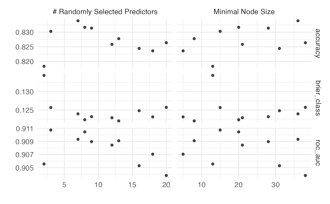
⏱️ Your Turn 4

Here’s our random forest model plus workflow to work with.

rf_mod <- rand_forest(engine = "ranger") |>
  set_mode("classification")

rf_wf <- workflow() |>
  add_formula(children ~ .) |>
  add_model(rf_mod)

⏱️ Your Turn 4

Here is the output from fit_resamples()…

set.seed(100) # Important!
rf_results <- rf_wf |>
  fit_resamples(resamples = hotels_folds)

rf_results |>
  collect_metrics()

# A tibble: 3 × 6
  .metric     .estimator  mean     n std_err .config        
  <chr>       <chr>      <dbl> <int>   <dbl> <chr>          
1 accuracy    binary     0.832    10 0.00576 Preprocessor1_…
2 brier_class binary     0.122    10 0.00224 Preprocessor1_…
3 roc_auc     binary     0.913    10 0.00382 Preprocessor1_…

⏱️ Your Turn 4

Edit the random forest model to tune the mtry and min_n hyperparameters.

Update your workflow to use the tuned model.

Then use tune_grid() to find the best combination of hyper-parameters to maximize roc_auc; let tune set up the grid for you.

How does it compare to the average ROC AUC across folds from fit_resamples()?

05:00

rf_tuner <- rand_forest(
  engine = "ranger",
  mtry = tune(),
  min_n = tune()
) |>
  set_mode("classification")

rf_wf <- rf_wf |>
  update_model(rf_tuner)

set.seed(100) # Important!
rf_results <- rf_wf |>
  tune_grid(
    resamples = hotels_folds,
    control = control_grid(save_workflow = TRUE)
  )

rf_results |>
  collect_metrics()

# A tibble: 30 × 8
    mtry min_n .metric     .estimator  mean     n std_err
   <int> <int> <chr>       <chr>      <dbl> <int>   <dbl>
 1     9    28 accuracy    binary     0.831    10 0.00506
 2     9    28 brier_class binary     0.123    10 0.00231
 3     9    28 roc_auc     binary     0.909    10 0.00379
 4     7    36 accuracy    binary     0.834    10 0.00525
 5     7    36 brier_class binary     0.124    10 0.00220
 6     7    36 roc_auc     binary     0.909    10 0.00380
 7    12    21 accuracy    binary     0.826    10 0.00543
 8    12    21 brier_class binary     0.123    10 0.00238
 9    12    21 roc_auc     binary     0.908    10 0.00389
10     2    13 accuracy    binary     0.818    10 0.00672
# ℹ 20 more rows
# ℹ 1 more variable: .config <chr>

rf_results |>
  collect_metrics(summarize = FALSE)

# A tibble: 300 × 7
   id      mtry min_n .metric   .estimator .estimate .config
   <chr>  <int> <int> <chr>     <chr>          <dbl> <chr>  
 1 Fold01     9    28 accuracy  binary         0.825 Prepro…
 2 Fold01     9    28 roc_auc   binary         0.919 Prepro…
 3 Fold01     9    28 brier_cl… binary         0.117 Prepro…
 4 Fold02     9    28 accuracy  binary         0.842 Prepro…
 5 Fold02     9    28 roc_auc   binary         0.913 Prepro…
 6 Fold02     9    28 brier_cl… binary         0.121 Prepro…
 7 Fold03     9    28 accuracy  binary         0.847 Prepro…
 8 Fold03     9    28 roc_auc   binary         0.906 Prepro…
 9 Fold03     9    28 brier_cl… binary         0.123 Prepro…
10 Fold04     9    28 accuracy  binary         0.825 Prepro…
# ℹ 290 more rows

`tune_grid()`

A version of fit_resamples() that performs a grid search for the best combination of tuned hyper-parameters.

tune_grid(
  object,
  resamples,
  ...,
  grid = df,
  metrics = NULL,
  control = control_grid()
)

A data frame of tuning combinations.

`expand_grid()`

Takes one or more vectors, and returns a data frame holding all combinations of their values.

expand_grid(mtry = c(1, 5), min_n = 1:3)

# A tibble: 6 × 2
   mtry min_n
  <dbl> <int>
1     1     1
2     1     2
3     1     3
4     5     1
5     5     2
6     5     3

`show_best()`

Shows the n most optimum combinations of hyper-parameters

rf_results |>
  show_best(metric = "roc_auc", n = 5)

# A tibble: 5 × 8
   mtry min_n .metric .estimator  mean     n std_err .config
  <int> <int> <chr>   <chr>      <dbl> <int>   <dbl> <chr>  
1     3    15 roc_auc binary     0.911    10 0.00404 Prepro…
2     8    20 roc_auc binary     0.910    10 0.00405 Prepro…
3     7    36 roc_auc binary     0.909    10 0.00380 Prepro…
4    13     8 roc_auc binary     0.909    10 0.00393 Prepro…
5     9    28 roc_auc binary     0.909    10 0.00379 Prepro…

`autoplot()`

Quickly visualize tuning results

rf_results |> autoplot()

`fit_best()`

Replaces tune() placeholders in a model/recipe/workflow with a set of hyper-parameter values
Fits a model using the entire training set

last_rf_fit <- fit_best(rf_results, verbose = TRUE)

Using roc_auc as the metric, the optimal parameters were:
  mtry:  3
  min_n: 15

ℹ Fitting using 3600 data points...
✔ Done.

We are ready to touch the jewels…

The testing set!

⏱️ Your Turn 5

Use fit_best() to take the best combination of hyper-parameters from rf_results and use them to predict the test set.

How does our actual test ROC AUC compare to our cross-validated estimate?

05:00

hotels_best <- fit_best(rf_results)

# cross validated ROC AUC
rf_results |>
  show_best(metric = "roc_auc", n = 1)

# A tibble: 1 × 8
   mtry min_n .metric .estimator  mean     n std_err .config
  <int> <int> <chr>   <chr>      <dbl> <int>   <dbl> <chr>  
1     3    15 roc_auc binary     0.911    10 0.00404 Prepro…

# test set ROC AUC
bind_cols(
  hotels_test,
  predict(hotels_best, new_data = hotels_test, type = "prob")
) |>
  roc_auc(truth = children, .pred_children)

# A tibble: 1 × 3
  .metric .estimator .estimate
  <chr>   <chr>          <dbl>
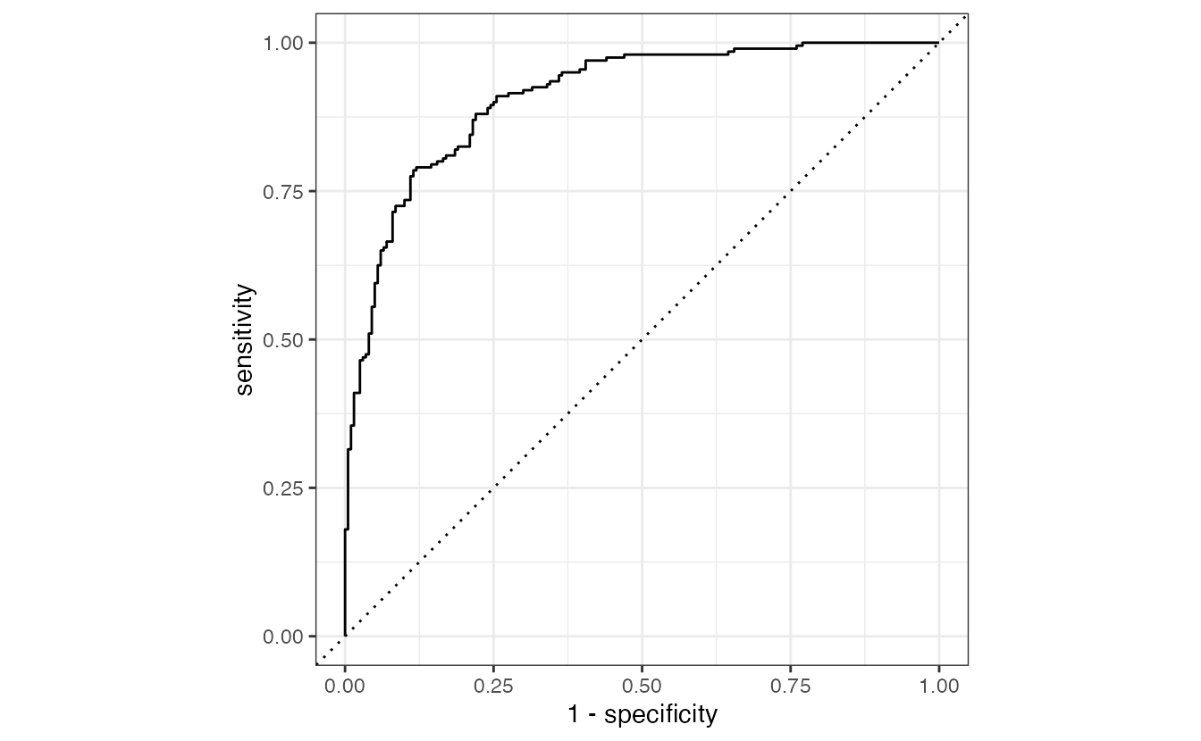
1 roc_auc binary         0.910

ROC curve

bind_cols(
  hotels_test,
  predict(hotels_best, new_data = hotels_test, type = "prob")
) |>
  roc_curve(truth = children, .pred_children) |>
  autoplot()

The entire process

The set-up

set.seed(100) # Important!

# holdout method
hotels_split <- initial_split(hotels, strata = children, prop = .9)
hotels_train <- training(hotels_split)
hotels_test <- testing(hotels_split)

# add cross-validation
set.seed(100)
hotels_folds <- vfold_cv(hotels_train, v = 10, strata = children)

The tune-up

# here comes the actual ML bits…

# pick model to tune
rf_tuner <- rand_forest(
  engine = "ranger",
  mtry = tune(),
  min_n = tune()
) |>
  set_mode("classification")

rf_wf <- workflow() |>
  add_formula(children ~ .) |>
  add_model(rf_tuner)

rf_results <- rf_wf |>
  tune_grid(
    resamples = hotels_folds,
    control = control_grid(
      save_pred = TRUE,
      save_workflow = TRUE
    )
  )

Quick check-in…

rf_results |>
  collect_predictions() |>
  group_by(.config, mtry, min_n) |>
  summarize(folds = n_distinct(id))

# A tibble: 10 × 4
# Groups:   .config, mtry [10]
   .config                mtry min_n folds
   <chr>                 <int> <int> <int>
 1 Preprocessor1_Model01     6    37    10
 2 Preprocessor1_Model02     9    35    10
 3 Preprocessor1_Model03     3    27    10
 4 Preprocessor1_Model04    15    18    10
 5 Preprocessor1_Model05    17    22    10
 6 Preprocessor1_Model06     9    15    10
 7 Preprocessor1_Model07     1     3    10
 8 Preprocessor1_Model08    13    10    10
 9 Preprocessor1_Model09    20    32    10
10 Preprocessor1_Model10    16     6    10

The match up!

show_best(rf_results, metric = "roc_auc", n = 5)

# A tibble: 5 × 8
   mtry min_n .metric .estimator  mean     n
  <int> <int> <chr>   <chr>      <dbl> <int>
1     9    15 roc_auc binary     0.910    10
2     6    37 roc_auc binary     0.910    10
3    13    10 roc_auc binary     0.909    10
4     3    27 roc_auc binary     0.909    10
5     9    35 roc_auc binary     0.908    10
# ℹ 2 more variables: std_err <dbl>,
#   .config <chr>

# pick final model workflow
hotels_best <- rf_results |>
  select_best(metric = "roc_auc")

hotels_best

# A tibble: 1 × 3
   mtry min_n .config              
  <int> <int> <chr>                
1     9    15 Preprocessor1_Model06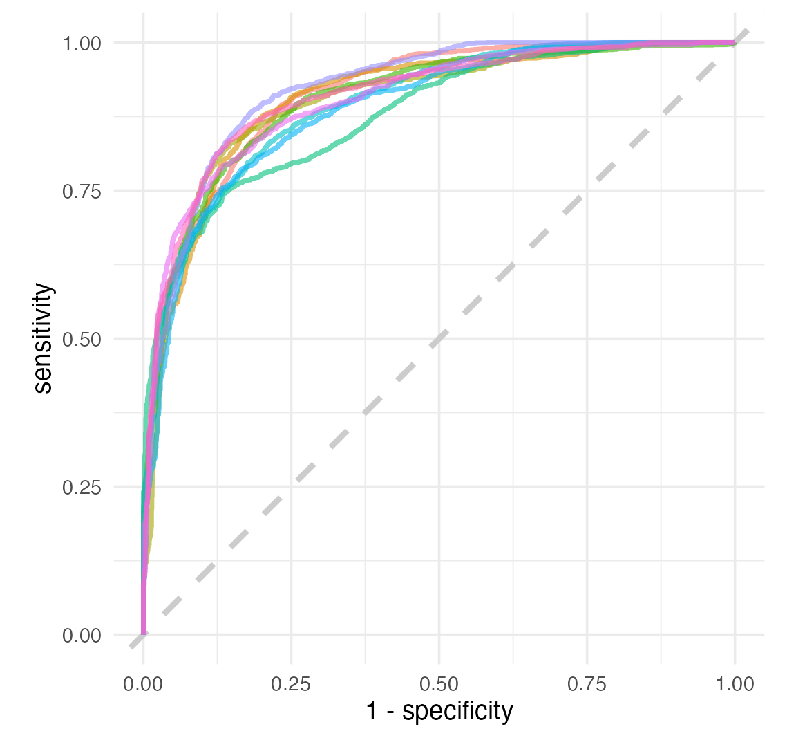

The wrap-up

# fit using best hyperparameter values
# and full training set
best_rf <- fit_best(rf_results)
best_rf

══ Workflow [trained] ══════════════════════════════════════════════════════════
Preprocessor: Formula
Model: rand_forest()

── Preprocessor ────────────────────────────────────────────────────────────────
children ~ .

── Model ───────────────────────────────────────────────────────────────────────
Ranger result

Call:
 ranger::ranger(x = maybe_data_frame(x), y = y, mtry = min_cols(~9L,      x), min.node.size = min_rows(~15L, x), num.threads = 1, verbose = FALSE,      seed = sample.int(10^5, 1), probability = TRUE) 

Type:                             Probability estimation 
Number of trees:                  500 
Sample size:                      3600 
Number of independent variables:  21 
Mtry:                             9 
Target node size:                 15 
Variable importance mode:         none 
Splitrule:                        gini 
OOB prediction error (Brier s.):  0.1209798

# predict probabilities for test set
bind_cols(
  hotels_test,
  predict(best_rf, new_data = hotels_test, type = "prob")
) |>
  # generate ROC curve
  roc_curve(truth = children, .pred_children) |>
  autoplot()

Recap

Decision trees are a nonlinear, naturally interactive model for classification and regression tasks
Simple decision trees can be easily interpreted, but also less accurate
Random forests are ensembles of decision trees used to aggregate predictions for improved performance
Models with hyperparameters require tuning in order to achieve optimal performance
Once the optimal model is achieved via cross-validation, fit the model a final time using the entire training set and evaluate its performance using the test set

Acknowledgments

Materials derived from Tidymodels, Virtually by Allison Hill and licensed under a Creative Commons Attribution-ShareAlike 4.0 International (CC BY-SA) License.
Dataset and some modeling steps derived from A predictive modeling case study and licensed under a Creative Commons Attribution-ShareAlike 4.0 International (CC BY-SA) License.

The committee meeting is in session

Tree-based inference and hyperparameter optimization

Announcements

Announcements

Application exercise

ae-22

Decision trees

Decision Trees

Quiz

Uses of decision trees

What makes a good guesser?

To specify a model with parsnip

To specify a decision tree model with parsnip

⏱️ Your turn 1

⏱️ Your turn 1

Model arguments

args()

decision_tree()

decision_tree()

set_args()

tree_depth

min_n

Quiz

Recap: early stopping

cost_complexity

Consider the bonsai

Consider the bonsai

Recap: early stopping & pruning

Axiom

Random forests

Ensemble methods

Bagging

Random forests

rand_forest()

rand_forest()

⏱️ Your turn 2

mtry

Single decision tree

A random forest of trees

⏱️ Your turn 3

🎶 Fitting and tuning models with tune

Hyperparameters

tune

tune()

tune_grid()

tune_grid()

tune_grid()

⏱️ Your Turn 4

⏱️ Your Turn 4

⏱️ Your Turn 4

tune_grid()

expand_grid()

show_best()

autoplot()

fit_best()

⏱️ Your Turn 5

ROC curve

The entire process

The set-up

The tune-up

Quick check-in…

The match up!

The wrap-up

Recap

Acknowledgments

The committee meeting is in session

`ae-22`

To specify a model with `parsnip`

To specify a decision tree model with `parsnip`

`args()`

`decision_tree()`

`decision_tree()`

`set_args()`

`tree_depth`

`min_n`

`cost_complexity`

`rand_forest()`

`rand_forest()`

`mtry`

🎶 Fitting and tuning models with `tune`

`tune`

`tune()`

`tune_grid()`

`tune_grid()`

`tune_grid()`

`tune_grid()`

`expand_grid()`

`show_best()`

`autoplot()`

`fit_best()`