library(tidyverse)
library(skimr)
library(scales)AE 06: Data types and classes
Application exercise
Answers
Packages
We will use the following packages in this application exercise.
- tidyverse: For data import, wrangling, and visualization.
- skimr: For summarizing the entire data frame at once.
- scales: For better axis labels.
Recoding survey results
Demo: Suppose you conducted a survey where you asked people how many cars their household owns collectively. And the answers are as follows:
survey_results <- tibble(cars = c(1, 2, "three"))
survey_results
# A tibble: 3 × 1
cars
<chr>
1 1
2 2
3 threeThis is annoying because of that third survey taker who just had to go and type out the number instead of providing as a numeric value. So now you need to update the cars variable to be numeric. You do the following
survey_results |>
  mutate(cars = as.numeric(cars))
Warning: There was 1 warning in `mutate()`.
ℹ In argument: `cars = as.numeric(cars)`.
Caused by warning:
! NAs introduced by coercion# A tibble: 3 × 1
cars
<dbl>
1 1
2 2
3 NAAnd now things are even more annoying because you get a warning NAs introduced by coercion that happened while computing cars = as.numeric(cars) and the response from the third survey taker is now an NA (you lost their data). Fix your mutate() call to avoid this warning.
survey_results |>
  mutate(
    cars = if_else(cars == "three", "3", cars),
    cars = as.numeric(cars)
  )
# A tibble: 3 × 1
cars
<dbl>
1 1
2 2
3 3# or with parse_number()
survey_results |>
mutate(
cars = if_else(cars == "three", "3", cars),
cars = parse_number(cars)
)# A tibble: 3 × 1
cars
<dbl>
1 1
2 2
3 3Hotel bookings
Antonio, Almeida, and Nunes (2019) collected detailed information on hotel bookings from two hotels (one resort hotel and one city hotel) in Portugal. The data set contains information such as when the booking was made, length of stay, number of adults, number of children, and number of available parking spaces.
Load the data
The data is stored in data/hotels-tt.csv. Let’s load the data file and examine it’s contents. Since the dataset is substantially large (nearly 30 variables and over 100,000 observations), we’ll use skimr::skim() to provide a compact summary of the data.
hotels <- read_csv("data/hotels-tt.csv")
skim(hotels) # much more useful to run interactively in the console| Name | hotels |
| Number of rows | 119390 |
| Number of columns | 29 |
| _______________________ | |
| Column type frequency: | |
| character | 13 |
| Date | 1 |
| numeric | 15 |
| ________________________ | |
| Group variables | None |
Variable type: character
| skim_variable | n_missing | complete_rate | min | max | empty | n_unique | whitespace |
|---|---|---|---|---|---|---|---|
| hotel | 0 | 1 | 10 | 12 | 0 | 2 | 0 |
| arrival_date | 0 | 1 | 11 | 18 | 0 | 793 | 0 |
| meal | 0 | 1 | 2 | 9 | 0 | 5 | 0 |
| country | 0 | 1 | 2 | 4 | 0 | 178 | 0 |
| market_segment | 0 | 1 | 6 | 13 | 0 | 8 | 0 |
| distribution_channel | 0 | 1 | 3 | 9 | 0 | 5 | 0 |
| reserved_room_type | 0 | 1 | 1 | 1 | 0 | 10 | 0 |
| assigned_room_type | 0 | 1 | 1 | 1 | 0 | 12 | 0 |
| deposit_type | 0 | 1 | 10 | 10 | 0 | 3 | 0 |
| agent | 0 | 1 | 1 | 4 | 0 | 334 | 0 |
| company | 0 | 1 | 1 | 4 | 0 | 353 | 0 |
| customer_type | 0 | 1 | 5 | 15 | 0 | 4 | 0 |
| reservation_status | 0 | 1 | 7 | 9 | 0 | 3 | 0 |
Variable type: Date
| skim_variable | n_missing | complete_rate | min | max | median | n_unique |
|---|---|---|---|---|---|---|
| reservation_status_date | 0 | 1 | 2014-10-17 | 2017-09-14 | 2016-08-07 | 926 |
Variable type: numeric
| skim_variable | n_missing | complete_rate | mean | sd | p0 | p25 | p50 | p75 | p100 | hist |
|---|---|---|---|---|---|---|---|---|---|---|
| is_canceled | 0 | 1 | 0.37 | 0.48 | 0.00 | 0.00 | 0.00 | 1 | 1 | ▇▁▁▁▅ |
| lead_time | 0 | 1 | 104.01 | 106.86 | 0.00 | 18.00 | 69.00 | 160 | 737 | ▇▂▁▁▁ |
| stays_in_weekend_nights | 0 | 1 | 0.93 | 1.00 | 0.00 | 0.00 | 1.00 | 2 | 19 | ▇▁▁▁▁ |
| stays_in_week_nights | 0 | 1 | 2.50 | 1.91 | 0.00 | 1.00 | 2.00 | 3 | 50 | ▇▁▁▁▁ |
| adults | 0 | 1 | 1.86 | 0.58 | 0.00 | 2.00 | 2.00 | 2 | 55 | ▇▁▁▁▁ |
| children | 4 | 1 | 0.10 | 0.40 | 0.00 | 0.00 | 0.00 | 0 | 10 | ▇▁▁▁▁ |
| babies | 0 | 1 | 0.01 | 0.10 | 0.00 | 0.00 | 0.00 | 0 | 10 | ▇▁▁▁▁ |
| is_repeated_guest | 0 | 1 | 0.03 | 0.18 | 0.00 | 0.00 | 0.00 | 0 | 1 | ▇▁▁▁▁ |
| previous_cancellations | 0 | 1 | 0.09 | 0.84 | 0.00 | 0.00 | 0.00 | 0 | 26 | ▇▁▁▁▁ |
| previous_bookings_not_canceled | 0 | 1 | 0.14 | 1.50 | 0.00 | 0.00 | 0.00 | 0 | 72 | ▇▁▁▁▁ |
| booking_changes | 0 | 1 | 0.22 | 0.65 | 0.00 | 0.00 | 0.00 | 0 | 21 | ▇▁▁▁▁ |
| days_in_waiting_list | 0 | 1 | 2.32 | 17.59 | 0.00 | 0.00 | 0.00 | 0 | 391 | ▇▁▁▁▁ |
| adr | 0 | 1 | 101.83 | 50.54 | -6.38 | 69.29 | 94.58 | 126 | 5400 | ▇▁▁▁▁ |
| required_car_parking_spaces | 0 | 1 | 0.06 | 0.25 | 0.00 | 0.00 | 0.00 | 0 | 8 | ▇▁▁▁▁ |
| total_of_special_requests | 0 | 1 | 0.57 | 0.79 | 0.00 | 0.00 | 0.00 | 1 | 5 | ▇▁▁▁▁ |
How does the Average Daily Rate (ADR) change over time? Are there differences between the city and resort hotel?
Your turn: Create a visualization that shows the average daily rate (ADR) over time for the city and resort hotels. Calculate the average (mean) ADR for each hotel by month based on when the guest(s) are scheduled to arrive, then visualize using a line graph. Ensure the \(x\)-axis is ordered chronologically.
Note
Use the lubridate package to restructure the data and determine the month when each stay began.
hotels |>
  # generate month variable using lubridate
  mutate(arrival_date = mdy(arrival_date),
         arrival_date_month = month(arrival_date, label = TRUE),
         .after = arrival_date) |>
  group_by(hotel, arrival_date_month) |>
  summarize(mean_adr = mean(adr), .groups = "drop") |>
  ggplot(mapping = aes(
    x = arrival_date_month,
    y = mean_adr,
    group = hotel,
    color = hotel
  )) +
  geom_line() +
  scale_y_continuous(labels = label_dollar()) +
  scale_color_viridis_d(end = 0.8) +
  theme_minimal() +
  labs(
    x = "Arrival month",
    y = "Mean ADR (average daily rate)",
    title = "Comparison of resort and city hotel prices across months",
    subtitle = "Resort hotel prices soar in the summer while city hotel prices\nremain relatively constant throughout the year",
    color = "Hotel type"
  )
How often is each meal package booked?
Your turn: meal reports the type of meal booked with the hotel stay. Categories are presented in standard hospitality meal packages:
Undefined/SC– no meal packageBB– Bed & BreakfastHB– Half board (breakfast and one other meal – usually dinner)FB– Full board (breakfast, lunch and dinner)
Create a bar chart reporting the total number of bookings for each meal package. Order the bars by frequency (i.e. most frequent meal package on the left, least frequent meal package on the right).
Note
forcats will be your friend in preparing the data for the visualization.
# create plot without summarizing the data frame
hotels |>
  mutate(
    # convert to factor column
    meal = factor(x = meal),
    # recode levels to human-readable, collapsing Undefined and SC simultaneously
    meal = fct_recode(.f = meal,
                      `No meal package` = "Undefined",
                      `No meal package` = "SC",
                      `Bed & Breakfast` = "BB",
                      `Half board` = "HB",
                      `Full board` = "FB"),
    # order by frequency
    meal = fct_infreq(f = meal)
  ) |>
  ggplot(mapping = aes(x = meal)) +
  geom_bar() +
  scale_y_continuous(labels = label_comma()) +
  labs(
    x = "Meal package",
    y = "Number of bookings",
    title = "Most bookings are for a bed and breakfast package"
  ) +
  theme_minimal()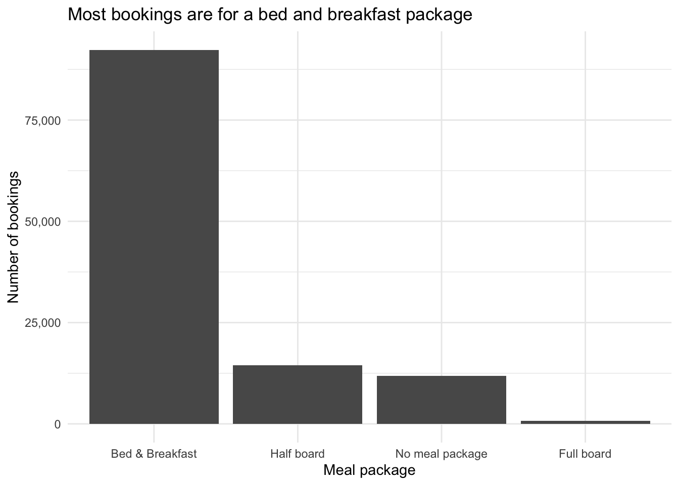
# create plot by summarizing the data frame
hotels |>
  mutate(
    # convert to factor column
    meal = factor(x = meal),
    # recode levels to human-readable, collapsing Undefined and SC simultaneously
    meal = fct_recode(.f = meal,
                      `No meal package` = "Undefined",
                      `No meal package` = "SC",
                      `Bed & Breakfast` = "BB",
                      `Half board` = "HB",
                      `Full board` = "FB")
  ) |>
  # generate frequency count table
  count(meal) |>
  # reorder meal based on the n column
  # need to reverse the order so it plots correctly
  mutate(meal = fct_reorder(.f = meal, .x = n, .desc = TRUE)) |>
  ggplot(mapping = aes(x = meal, y = n)) +
  geom_col() +
  scale_y_continuous(labels = label_comma()) +
  labs(
    x = "Meal package",
    y = "Number of bookings",
    title = "Most bookings are for a bed and breakfast package"
  ) +
  theme_minimal()
Session information
sessioninfo::session_info()─ Session info ───────────────────────────────────────────────────────────────
setting value
version R version 4.3.2 (2023-10-31)
os macOS Ventura 13.5.2
system aarch64, darwin20
ui X11
language (EN)
collate en_US.UTF-8
ctype en_US.UTF-8
tz America/New_York
date 2024-02-17
pandoc 3.1.1 @ /Applications/RStudio.app/Contents/Resources/app/quarto/bin/tools/ (via rmarkdown)
─ Packages ───────────────────────────────────────────────────────────────────
package * version date (UTC) lib source
base64enc 0.1-3 2015-07-28 [1] CRAN (R 4.3.0)
bit 4.0.5 2022-11-15 [1] CRAN (R 4.3.0)
bit64 4.0.5 2020-08-30 [1] CRAN (R 4.3.0)
cli 3.6.2 2023-12-11 [1] CRAN (R 4.3.1)
colorspace 2.1-0 2023-01-23 [1] CRAN (R 4.3.0)
crayon 1.5.2 2022-09-29 [1] CRAN (R 4.3.0)
digest 0.6.34 2024-01-11 [1] CRAN (R 4.3.1)
dplyr * 1.1.4 2023-11-17 [1] CRAN (R 4.3.1)
evaluate 0.23 2023-11-01 [1] CRAN (R 4.3.1)
fansi 1.0.6 2023-12-08 [1] CRAN (R 4.3.1)
farver 2.1.1 2022-07-06 [1] CRAN (R 4.3.0)
fastmap 1.1.1 2023-02-24 [1] CRAN (R 4.3.0)
forcats * 1.0.0 2023-01-29 [1] CRAN (R 4.3.0)
generics 0.1.3 2022-07-05 [1] CRAN (R 4.3.0)
ggplot2 * 3.4.4 2023-10-12 [1] CRAN (R 4.3.1)
glue 1.7.0 2024-01-09 [1] CRAN (R 4.3.1)
gtable 0.3.4 2023-08-21 [1] CRAN (R 4.3.0)
here 1.0.1 2020-12-13 [1] CRAN (R 4.3.0)
hms 1.1.3 2023-03-21 [1] CRAN (R 4.3.0)
htmltools 0.5.7 2023-11-03 [1] CRAN (R 4.3.1)
htmlwidgets 1.6.4 2023-12-06 [1] CRAN (R 4.3.1)
jsonlite 1.8.8 2023-12-04 [1] CRAN (R 4.3.1)
knitr 1.45 2023-10-30 [1] CRAN (R 4.3.1)
labeling 0.4.3 2023-08-29 [1] CRAN (R 4.3.0)
lifecycle 1.0.4 2023-11-07 [1] CRAN (R 4.3.1)
lubridate * 1.9.3 2023-09-27 [1] CRAN (R 4.3.1)
magrittr 2.0.3 2022-03-30 [1] CRAN (R 4.3.0)
munsell 0.5.0 2018-06-12 [1] CRAN (R 4.3.0)
pillar 1.9.0 2023-03-22 [1] CRAN (R 4.3.0)
pkgconfig 2.0.3 2019-09-22 [1] CRAN (R 4.3.0)
purrr * 1.0.2 2023-08-10 [1] CRAN (R 4.3.0)
R6 2.5.1 2021-08-19 [1] CRAN (R 4.3.0)
readr * 2.1.5 2024-01-10 [1] CRAN (R 4.3.1)
repr 1.1.6 2023-01-26 [1] CRAN (R 4.3.0)
rlang 1.1.3 2024-01-10 [1] CRAN (R 4.3.1)
rmarkdown 2.25 2023-09-18 [1] CRAN (R 4.3.1)
rprojroot 2.0.4 2023-11-05 [1] CRAN (R 4.3.1)
rstudioapi 0.15.0 2023-07-07 [1] CRAN (R 4.3.0)
scales * 1.2.1 2024-01-18 [1] Github (r-lib/scales@c8eb772)
sessioninfo 1.2.2 2021-12-06 [1] CRAN (R 4.3.0)
skimr * 2.1.5 2022-12-23 [1] CRAN (R 4.3.0)
stringi 1.8.3 2023-12-11 [1] CRAN (R 4.3.1)
stringr * 1.5.1 2023-11-14 [1] CRAN (R 4.3.1)
tibble * 3.2.1 2023-03-20 [1] CRAN (R 4.3.0)
tidyr * 1.3.0 2023-01-24 [1] CRAN (R 4.3.0)
tidyselect 1.2.0 2022-10-10 [1] CRAN (R 4.3.0)
tidyverse * 2.0.0 2023-02-22 [1] CRAN (R 4.3.0)
timechange 0.2.0 2023-01-11 [1] CRAN (R 4.3.0)
tzdb 0.4.0 2023-05-12 [1] CRAN (R 4.3.0)
utf8 1.2.4 2023-10-22 [1] CRAN (R 4.3.1)
vctrs 0.6.5 2023-12-01 [1] CRAN (R 4.3.1)
viridisLite 0.4.2 2023-05-02 [1] CRAN (R 4.3.0)
vroom 1.6.5 2023-12-05 [1] CRAN (R 4.3.1)
withr 2.5.2 2023-10-30 [1] CRAN (R 4.3.1)
xfun 0.41 2023-11-01 [1] CRAN (R 4.3.1)
yaml 2.3.8 2023-12-11 [1] CRAN (R 4.3.1)
[1] /Library/Frameworks/R.framework/Versions/4.3-arm64/Resources/library
──────────────────────────────────────────────────────────────────────────────