library(tidyverse)
library(jsonlite)AE 13: Rectangling data from the PokéAPI
Suggested answers
Application exercise
Answers
Packages
We will use the following packages in this application exercise.
- tidyverse: For data import, wrangling, and visualization.
- jsonlite: For importing JSON files
Gotta catch em’ all!
Pokémon (also known as Pocket Monsters) is a Japanese media franchise consisting of video games, animated series and films, a trading card game, and other related media.1 The PokéAPI contains detailed information about each Pokémon, including their name, type, and abilities. In this application exercise, we will use a set of JSON files containing API results from the PokéAPI to explore the Pokémon universe.
Importing the data
data/pokedex.json and data/types.json contain information about each Pokémon and the different types of Pokémon, respectively. We will use read_json() to import these files.
pokemon <- read_json(path = "data/pokemon/pokedex.json")
types <- read_json(path = "data/pokemon/types.json")
Your turn: Use View() to interactively explore each list object to identify their structure and the elements contained within each object.
Unnesting for analysis
For each of the exercises below, use an appropriate rectangling procedure to unnest_*() one or more lists to extract the required elements for analysis.
How many Pokémon are there for each primary type?
Your turn: Use each Pokemon’s primary type (the first one listed in the data) to determine how many Pokémon there are for each type, then create a bar chart to visualize the distribution.
Tip
Examine the contents of each list object to determine how the relevant variables are structured so you can plan your approach.
There are (at least) three ways you could approach this problem.
- Use
unnest_wider()twice to extract the primary type from the pokemon list and generate a frequency count. - Use
unnest_wider()andhoist()to extract the primary type from the pokemon list and generate a frequency count. - Use
unnest_wider()andunnest_longer()to extract the primary type from the pokemon list and generate a frequency count.
Pick one and have at it!
Note
Fancy a challenge? Label each Pokémon type in both English and Japanese.
# extract the primary type from the pokemon list and generate a frequency count
## using hoist()
poke_types <- tibble(pokemon) |>
  # expand so each pokemon variable is in its own column
  unnest_wider(pokemon) |>
  # extract the pokemon's primary type from the type column
  hoist(.col = type, main_type = 1L) |>
  # generate frequency count
  count(main_type)

## using unnest_wider() twice
poke_types <- tibble(pokemon) |>
  # expand so each pokemon variable is in its own column
  unnest_wider(pokemon) |>
  # expand the type column so each type is in its own column
  unnest_wider(type, names_sep = "_") |>
  rename(main_type = type_1) |>
  # generate frequency count
  count(main_type)

## using unnest_wider() and unnest_longer()
poke_types <- tibble(pokemon) |>
  # expand so each pokemon variable is in its own column
  unnest_wider(pokemon) |>
  # expand the type column so each type is in its own row
  unnest_longer(type) |>
  # keep just the first row for each pokemon
  slice_head(n = 1, by = id) |>
  # generate frequency count
  count(main_type = type)

# extract english and japanese names for types
types_df <- tibble(types) |>
  unnest_wider(types)

# combine poke_types with types_df and create a name column that includes both
# english and japanese
left_join(x = poke_types, y = types_df, by = join_by(main_type == english)) |>
  mutate(
    name = str_glue("{main_type} ({japanese})"),
    name = fct_reorder(.f = name, .x = n)
  ) |>
  ggplot(mapping = aes(x = n, y = name)) +
  geom_col() +
  labs(
    title = "Water-type Pokémon are the most common",
    x = "Number of Pokémon",
    y = NULL,
    caption = "Source: PokéAPI"
  ) +
  theme_minimal()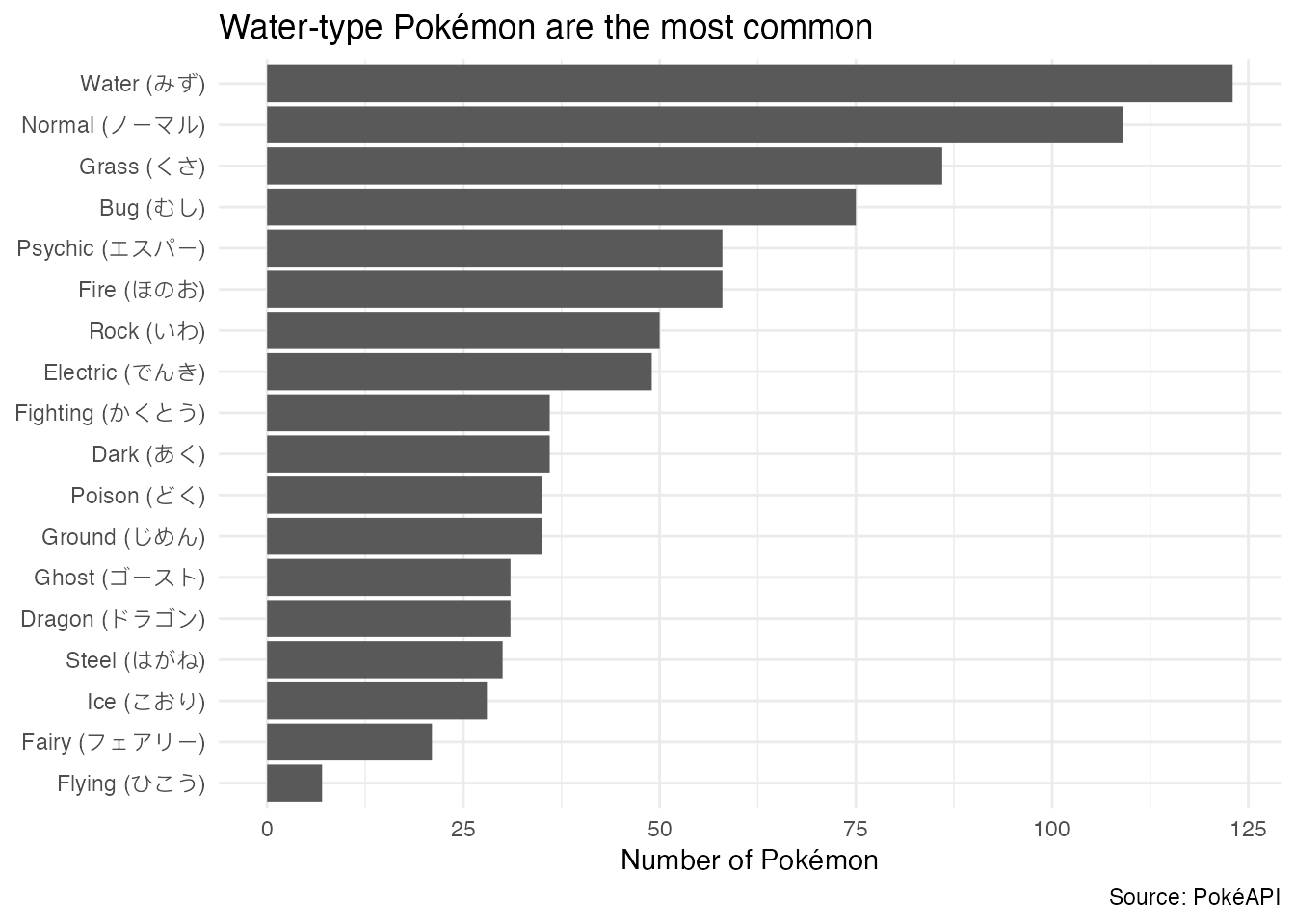
Which primary type of Pokémon are strongest based on total number of points?
Your turn: Use each Pokémon’s base stats to determine which primary type of Pokémon are strongest based on the total number of points. Create a boxplot to visualize the distribution of total points for each primary type.
Tip
To calculate the sum total of points for each Pokémon’s base stats, there are two approaches you might consider. In either approach you first need to get each Pokémon’s variables into separate columns and extract the primary type.
- Use
unnest_wider()to extract the base stats, then calculate the sum of the base stats. - Use
unnest_longer()to extract the base stats, then calculate the sum of the base stats.
# base stats in one column per stat
pokemon_points <- tibble(pokemon) |>
  # one column per variable
  unnest_wider(pokemon) |>
  # extract the pokemon's primary type from the type column
  hoist(.col = type, main_type = 1L) |>
  # expand to get base stats
  unnest_wider(base) |>
  # for each row, calculate the sum of HP:Speed
  rowwise() |>
  mutate(total = sum(c_across(cols = HP:Speed), na.rm = TRUE), .before = HP) |>
  ungroup() |>
  # exclude pokemon with total = 0 - means we don't have stats available
  filter(total != 0) |>
  select(id, main_type, total)
pokemon_points
# A tibble: 809 × 3
id main_type total
<int> <chr> <int>
1 1 Grass 318
2 2 Grass 405
3 3 Grass 525
4 4 Fire 309
5 5 Fire 405
6 6 Fire 534
7 7 Water 314
8 8 Water 405
9 9 Water 530
10 10 Bug 195
# ℹ 799 more rows# base stats in one row per pokemon per stat
pokemon_points <- tibble(pokemon) |>
# one column per variable
unnest_wider(pokemon) |>
# extract the pokemon's primary type from the type column
hoist(.col = type, main_type = 1L) |>
# expand to get base stats
unnest_longer(base,
values_to = "points",
indices_to = "stat"
) |>
# calculate sum of points for each pokemon
summarize(total = sum(points, na.rm = TRUE), .by = c(id, main_type))
pokemon_points# A tibble: 809 × 3
id main_type total
<int> <chr> <int>
1 1 Grass 318
2 2 Grass 405
3 3 Grass 525
4 4 Fire 309
5 5 Fire 405
6 6 Fire 534
7 7 Water 314
8 8 Water 405
9 9 Water 530
10 10 Bug 195
# ℹ 799 more rowspokemon_points |>
# order the boxplots meaningfully
mutate(main_type = fct_reorder(.f = main_type, .x = total)) |>
# generate the plot
ggplot(mapping = aes(x = total, y = main_type)) +
geom_boxplot() +
labs(
title = "Flying-type Pokémon are the most powerful on average",
x = "Total points",
y = NULL,
caption = "Source: PokéAPI"
) +
theme_minimal()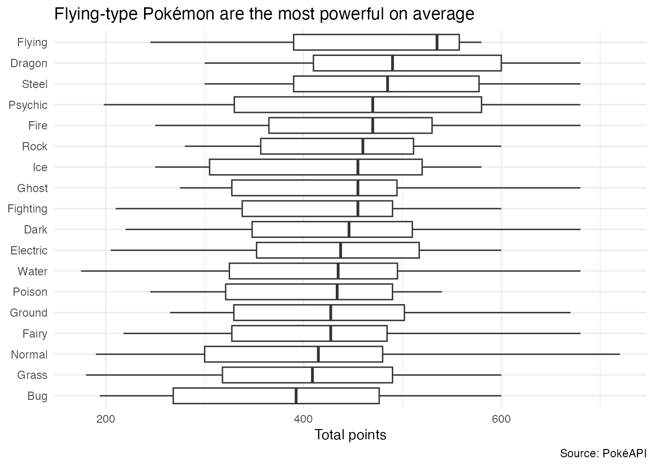
From what types of eggs do Pokémon hatch? (Bonus!)
In Generation II, Pokémon introduced the concept of breeding, whereby Pokémon can produce offspring. In Generation III, Pokémon eggs were introduced, which can be hatched to produce a Pokémon.

Use each Pokémon’s egg group to determine from what types of eggs Pokémon hatch. Create a heatmap like the one below to visualize the distribution of egg groups for each primary type.

Tip
Consider using hoist() to extract the main type and egg group from each Pokémon.
tibble(pokemon) |>
  unnest_wider(pokemon) |>
  # extract the main type
  hoist(
    .col = type, main_type = 1L
  ) |>
  # extract the type of eggs from which the pokemon can hatch
  hoist(
    .col = profile, egg = "egg"
  ) |>
  select(main_type, egg) |>
  # some pokemon have more than one egg group, need to unnest longer
  unnest_longer(egg) |>
  # count the number of type-egg pairings
  count(main_type, egg) |>
  # draw the plot
  ggplot(mapping = aes(x = egg, y = main_type, fill = n)) +
  geom_tile() +
  geom_text(mapping = aes(label = n), color = "white") +
  scale_fill_viridis_c() +
  theme_minimal() +
  labs(
    title = "A few Pokémon types are more likely to hatch from certain eggs",
    x = "Egg group",
    y = "Main Pokémon type",
    caption = "Source: PokéAPI"
  ) +
  theme(
    legend.position = "none",
    axis.text.x = element_text(angle = 30, hjust = 1)
  )
Acknowledgments
- JSON data files obtained from
Purukitto/pokemon-data.json
Session information
sessioninfo::session_info()─ Session info ───────────────────────────────────────────────────────────────
setting value
version R version 4.3.2 (2023-10-31)
os macOS Ventura 13.5.2
system aarch64, darwin20
ui X11
language (EN)
collate en_US.UTF-8
ctype en_US.UTF-8
tz America/New_York
date 2024-03-16
pandoc 3.1.1 @ /Applications/RStudio.app/Contents/Resources/app/quarto/bin/tools/ (via rmarkdown)
─ Packages ───────────────────────────────────────────────────────────────────
package * version date (UTC) lib source
cli 3.6.2 2023-12-11 [1] CRAN (R 4.3.1)
colorspace 2.1-0 2023-01-23 [1] CRAN (R 4.3.0)
digest 0.6.34 2024-01-11 [1] CRAN (R 4.3.1)
dplyr * 1.1.4 2023-11-17 [1] CRAN (R 4.3.1)
evaluate 0.23 2023-11-01 [1] CRAN (R 4.3.1)
fansi 1.0.6 2023-12-08 [1] CRAN (R 4.3.1)
farver 2.1.1 2022-07-06 [1] CRAN (R 4.3.0)
fastmap 1.1.1 2023-02-24 [1] CRAN (R 4.3.0)
forcats * 1.0.0 2023-01-29 [1] CRAN (R 4.3.0)
generics 0.1.3 2022-07-05 [1] CRAN (R 4.3.0)
ggplot2 * 3.4.4 2023-10-12 [1] CRAN (R 4.3.1)
glue 1.7.0 2024-01-09 [1] CRAN (R 4.3.1)
gtable 0.3.4 2023-08-21 [1] CRAN (R 4.3.0)
here 1.0.1 2020-12-13 [1] CRAN (R 4.3.0)
hms 1.1.3 2023-03-21 [1] CRAN (R 4.3.0)
htmltools 0.5.7 2023-11-03 [1] CRAN (R 4.3.1)
htmlwidgets 1.6.4 2023-12-06 [1] CRAN (R 4.3.1)
jsonlite * 1.8.8 2023-12-04 [1] CRAN (R 4.3.1)
knitr 1.45 2023-10-30 [1] CRAN (R 4.3.1)
labeling 0.4.3 2023-08-29 [1] CRAN (R 4.3.0)
lifecycle 1.0.4 2023-11-07 [1] CRAN (R 4.3.1)
lubridate * 1.9.3 2023-09-27 [1] CRAN (R 4.3.1)
magrittr 2.0.3 2022-03-30 [1] CRAN (R 4.3.0)
munsell 0.5.0 2018-06-12 [1] CRAN (R 4.3.0)
pillar 1.9.0 2023-03-22 [1] CRAN (R 4.3.0)
pkgconfig 2.0.3 2019-09-22 [1] CRAN (R 4.3.0)
purrr * 1.0.2 2023-08-10 [1] CRAN (R 4.3.0)
R6 2.5.1 2021-08-19 [1] CRAN (R 4.3.0)
ragg 1.2.7 2023-12-11 [1] CRAN (R 4.3.1)
readr * 2.1.5 2024-01-10 [1] CRAN (R 4.3.1)
rlang 1.1.3 2024-01-10 [1] CRAN (R 4.3.1)
rmarkdown 2.25 2023-09-18 [1] CRAN (R 4.3.1)
rprojroot 2.0.4 2023-11-05 [1] CRAN (R 4.3.1)
rstudioapi 0.15.0 2023-07-07 [1] CRAN (R 4.3.0)
scales 1.2.1 2024-01-18 [1] Github (r-lib/scales@c8eb772)
sessioninfo 1.2.2 2021-12-06 [1] CRAN (R 4.3.0)
stringi 1.8.3 2023-12-11 [1] CRAN (R 4.3.1)
stringr * 1.5.1 2023-11-14 [1] CRAN (R 4.3.1)
systemfonts 1.0.5 2023-10-09 [1] CRAN (R 4.3.1)
textshaping 0.3.7 2023-10-09 [1] CRAN (R 4.3.1)
tibble * 3.2.1 2023-03-20 [1] CRAN (R 4.3.0)
tidyr * 1.3.0 2023-01-24 [1] CRAN (R 4.3.0)
tidyselect 1.2.0 2022-10-10 [1] CRAN (R 4.3.0)
tidyverse * 2.0.0 2023-02-22 [1] CRAN (R 4.3.0)
timechange 0.2.0 2023-01-11 [1] CRAN (R 4.3.0)
tzdb 0.4.0 2023-05-12 [1] CRAN (R 4.3.0)
utf8 1.2.4 2023-10-22 [1] CRAN (R 4.3.1)
vctrs 0.6.5 2023-12-01 [1] CRAN (R 4.3.1)
viridisLite 0.4.2 2023-05-02 [1] CRAN (R 4.3.0)
withr 2.5.2 2023-10-30 [1] CRAN (R 4.3.1)
xfun 0.41 2023-11-01 [1] CRAN (R 4.3.1)
yaml 2.3.8 2023-12-11 [1] CRAN (R 4.3.1)
[1] /Library/Frameworks/R.framework/Versions/4.3-arm64/Resources/library
──────────────────────────────────────────────────────────────────────────────