library(tidyverse)
library(tidymodels)
library(probably)
library(arthistory)
library(skimr)Gender representation in art history textbooks
Suggested answers
Application exercise
Answers
In this application exercise we will use logistic regression to predict the gender of artists with works included in Gardner’s Art Through the Ages, one of the most widely used art history textbooks in the United States. The data was originally compiled by Holland Stam for an undergraduate thesis.
The dataset is called worksgardner and can be found in the arthistory package, and we will use tidyverse and tidymodels for data exploration and modeling, respectively.
Please read the following context1 and take a skim of the data set before we get started.
This dataset contains data that was used for Holland Stam’s thesis work, titled Quantifying art historical narratives. The data was collected to assess the demographic representation of artists through editions of Janson’s History of Art and Gardner’s Art Through the Ages, two of the most popular art history textbooks used in the American education system. In this package specifically, both artist-level and work-level data was collected along with variables regarding the artists’ demographics and numeric metrics for describing how much space they or their work took up in each edition of each textbook.
worksgardner: Contains individual work-level data by edition of Gardner’s art history textbook from 1926 until 2020. For each work, there is information about the size of the work as displayed in the textbook as well as the size of the accompanying descriptive text. Demographic data about the artist is also included.
data("worksgardner")
skim(worksgardner)| Name | worksgardner |
| Number of rows | 2325 |
| Number of columns | 24 |
| _______________________ | |
| Column type frequency: | |
| character | 8 |
| numeric | 16 |
| ________________________ | |
| Group variables | None |
Variable type: character
| skim_variable | n_missing | complete_rate | min | max | empty | n_unique | whitespace |
|---|---|---|---|---|---|---|---|
| artist_name | 0 | 1 | 4 | 99 | 0 | 334 | 0 |
| title_of_work | 0 | 1 | 3 | 208 | 0 | 723 | 0 |
| page_number_of_image | 0 | 1 | 3 | 11 | 0 | 566 | 0 |
| artist_nationality | 0 | 1 | 3 | 18 | 0 | 49 | 0 |
| artist_gender | 0 | 1 | 3 | 6 | 0 | 3 | 0 |
| artist_race | 0 | 1 | 3 | 41 | 0 | 6 | 0 |
| artist_ethnicity | 0 | 1 | 3 | 22 | 0 | 3 | 0 |
| book | 0 | 1 | 7 | 7 | 0 | 1 | 0 |
Variable type: numeric
| skim_variable | n_missing | complete_rate | mean | sd | p0 | p25 | p50 | p75 | p100 | hist |
|---|---|---|---|---|---|---|---|---|---|---|
| edition_number | 0 | 1.00 | 10.29 | 4.02 | 1.00 | 7.00 | 11.00 | 14.00 | 16.00 | ▃▅▆▇▇ |
| publication_year | 0 | 1.00 | 1994.35 | 21.78 | 1926.00 | 1980.00 | 2001.00 | 2013.00 | 2020.00 | ▁▂▃▆▇ |
| artist_unique_id | 12 | 0.99 | 162.71 | 92.37 | 1.00 | 85.00 | 153.00 | 253.00 | 332.00 | ▆▇▇▇▆ |
| height_of_work_in_book | 0 | 1.00 | 10.95 | 3.12 | 0.00 | 9.00 | 10.70 | 12.40 | 25.40 | ▁▆▇▁▁ |
| width_of_work_in_book | 0 | 1.00 | 11.98 | 3.89 | 0.00 | 8.90 | 12.10 | 14.40 | 40.40 | ▁▇▂▁▁ |
| height_of_text | 0 | 1.00 | 13.55 | 8.13 | 0.00 | 8.00 | 11.90 | 16.80 | 63.20 | ▇▅▁▁▁ |
| width_of_text | 0 | 1.00 | 8.58 | 1.33 | 0.00 | 8.40 | 9.00 | 9.30 | 14.20 | ▁▁▅▇▁ |
| extra_text_height | 0 | 1.00 | 0.74 | 2.51 | 0.00 | 0.00 | 0.00 | 0.00 | 30.30 | ▇▁▁▁▁ |
| extra_text_width | 0 | 1.00 | 0.65 | 1.94 | 0.00 | 0.00 | 0.00 | 0.00 | 9.30 | ▇▁▁▁▁ |
| area_of_work_in_book | 0 | 1.00 | 133.62 | 60.97 | 0.00 | 98.04 | 123.28 | 157.92 | 495.51 | ▃▇▂▁▁ |
| area_of_text | 0 | 1.00 | 116.78 | 71.44 | 0.00 | 67.20 | 100.80 | 144.90 | 568.80 | ▇▅▁▁▁ |
| extra_text_area | 0 | 1.00 | 4.64 | 16.31 | 0.00 | 0.00 | 0.00 | 0.00 | 153.36 | ▇▁▁▁▁ |
| total_area_text | 0 | 1.00 | 121.45 | 72.13 | 0.00 | 72.00 | 105.00 | 149.40 | 568.80 | ▇▅▁▁▁ |
| total_space | 0 | 1.00 | 255.92 | 100.20 | 42.88 | 186.35 | 240.80 | 308.94 | 931.58 | ▆▇▁▁▁ |
| page_area | 0 | 1.00 | 584.23 | 107.17 | 203.04 | 568.48 | 646.70 | 651.84 | 677.44 | ▁▁▁▂▇ |
| space_ratio_per_page | 0 | 1.00 | 0.44 | 0.17 | 0.14 | 0.33 | 0.40 | 0.52 | 1.59 | ▇▅▁▁▁ |
Prep data for modeling
Before we attempt to model the data, first we will perform some data cleaning.
- Remove rows with
NAvalues or implausible values. - Convert
artist_genderto a factor column. - Log-transform
area_of_work_in_bookdue to skewness. - Lump infrequent nationalities into a single “Other” category.
works_subset <- worksgardner |>
  # remove rows with NAs or implausible values
  filter(
    artist_gender %in% c("Male", "Female"),
    area_of_work_in_book > 0,
    artist_race != "N/A",
    artist_ethnicity != "N/A"
  ) |>
  # minor feature engineering
  mutate(
    # convert artist_gender to factor column
    artist_gender = factor(artist_gender, levels = c("Male", "Female")),
    # log-transform area due to skewness
    area_of_work_in_book = log(area_of_work_in_book),
    # lump infrequent nationalities into a single "Other" category
    artist_nationality = fct_lump_n(f = artist_nationality, n = 6)
  ) |>
  # select columns for modeling
  select(
    artist_gender, publication_year, area_of_work_in_book,
    artist_nationality, artist_race, artist_ethnicity
  )
glimpse(works_subset)
Rows: 2,241
Columns: 6
$ artist_gender <fct> Male, Male, Male, Male, Male, Male, Male, Male, F…
$ publication_year <dbl> 1991, 1996, 2001, 2005, 2009, 2013, 2016, 2020, 2…
$ area_of_work_in_book <dbl> 4.564869, 4.679257, 4.684351, 4.684351, 4.779460,…
$ artist_nationality <fct> American, American, American, American, American,…
$ artist_race <chr> "Black or African American", "Black or African Am…
$ artist_ethnicity <chr> "Not Hispanic or Latinx", "Not Hispanic or Latinx…Split data into training/test sets
Demo: Now that we have cleaned the data, let’s split it into training and test sets. We will allocate 80% for training purposes (fitting a model) and 20% for testing purposes (evaluating model performance). Note the use of set.seed() so that every time we run the code we get the exact same split.
set.seed(123)

# split data into training and test sets
artist_split <- initial_split(data = works_subset, prop = 0.8)

# extract training/test sets as data frames
artist_train <- training(artist_split)
artist_test <- testing(artist_split)
Fit a simple logistic regression model
Your turn: Estimate a simple logistic regression model to predict the artist’s gender as a function of when the textbook was published.
# fit the logistic regression model
gender_year_fit <- logistic_reg() |>
  fit(artist_gender ~ publication_year, data = artist_train)
tidy(gender_year_fit)
# A tibble: 2 × 5
term estimate std.error statistic p.value
<chr> <dbl> <dbl> <dbl> <dbl>
1 (Intercept) -76.5 10.9 -7.00 2.55e-12
2 publication_year 0.0371 0.00545 6.81 9.73e-12What do the estimated parameters tell us at this point? Add response here.
Artists in textbooks published in later years are expected, on average, to be more likely female than in earlier years.
Visualize predicted probabilities
Your turn: Generate a plot to visualize the predicted probability that an artist is female based on the model estimated above.
# generate a sequence of years to predict
art_years <- tibble(
  publication_year = seq(
    from = min(works_subset$publication_year),
    to = max(works_subset$publication_year)
  )
)

# generate predicted probabilities
gender_year_pred <- predict(gender_year_fit, new_data = art_years, type = "prob") |>
  bind_cols(art_years)

# visualize predicted probabilities
ggplot(data = gender_year_pred, mapping = aes(x = publication_year, y = .pred_Female)) +
  geom_line() +
  scale_y_continuous(labels = label_percent()) +
  labs(
    x = "Publication year",
    y = "Predicted probability artist is female"
  )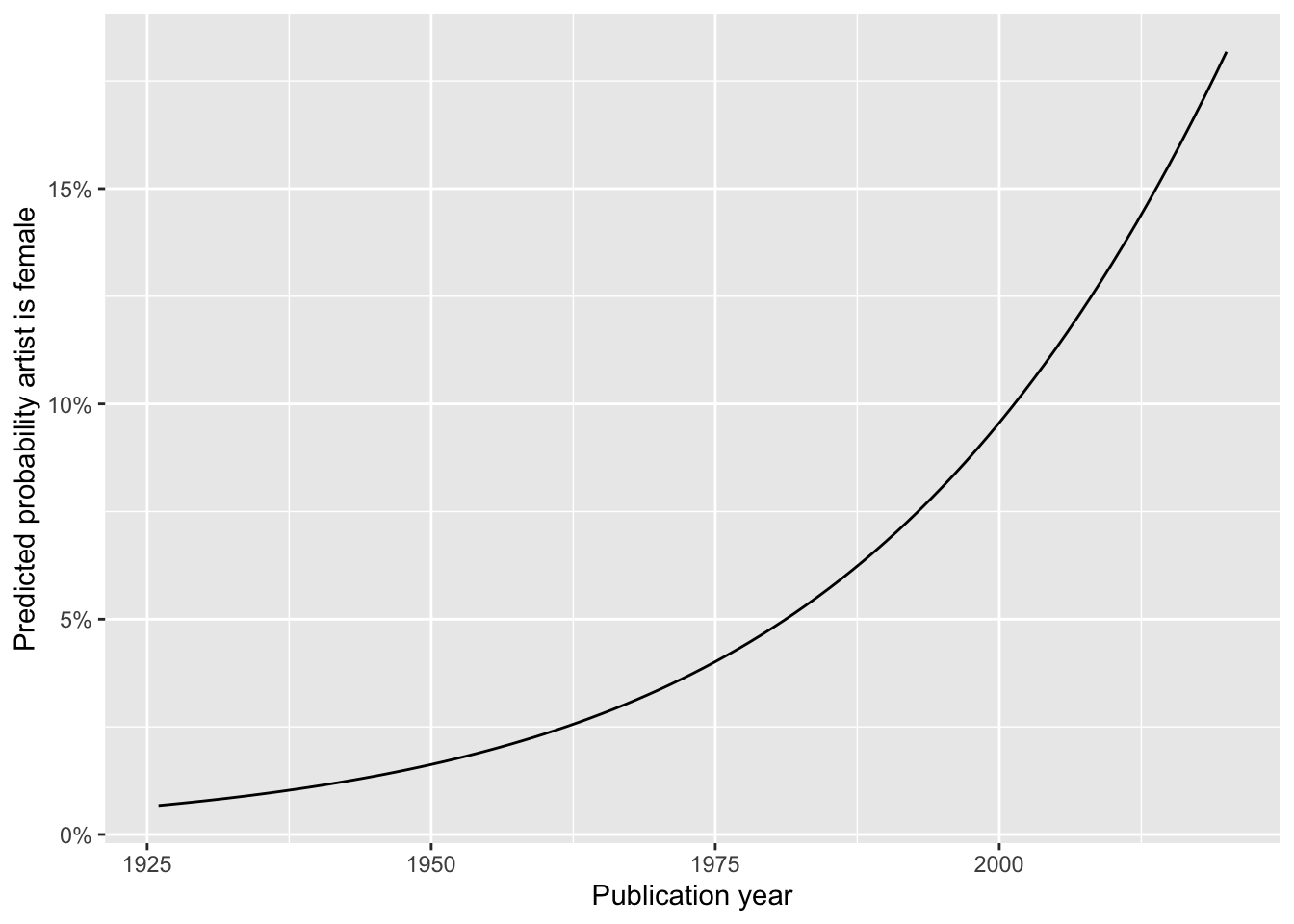
What are your takeaways? Add response here.
While the predicted probability that the artist is female is increasing over time, it is still very unlikely that the artist is female. Predicted probabilities are always below 20%.
Evaluate model’s performance
Demo: Estimate the model’s performance on the test set using metrics such as accuracy, confusion matrix, sensitivity, and specificity. What do you learn about the model’s performance?
# generate test set predictions
gender_year_pred <- predict(gender_year_fit, artist_test) |>
  bind_cols(artist_test |> select(artist_gender))

# model metrics
conf_mat(gender_year_pred, truth = artist_gender, .pred_class)
Truth
Prediction Male Female
Male 410 39
Female 0 0accuracy(gender_year_pred, truth = artist_gender, .pred_class)# A tibble: 1 × 3
.metric .estimator .estimate
<chr> <chr> <dbl>
1 accuracy binary 0.913sensitivity(gender_year_pred, truth = artist_gender, .pred_class)# A tibble: 1 × 3
.metric .estimator .estimate
<chr> <chr> <dbl>
1 sensitivity binary 1specificity(gender_year_pred, truth = artist_gender, .pred_class)# A tibble: 1 × 3
.metric .estimator .estimate
<chr> <chr> <dbl>
1 specificity binary 0Add response here.
This model does not perform well. It has a high accuracy, but this is due to the class imbalance in the data. The model is not able to predict the artist’s gender with any ability to discriminate between male and female artists. With a sensitivity of 0 and specificity of 1, the model is useless.
Fit a multiple variable logistic regression model
Your turn: Fit a multiple variable logistic regression model to predict the artist’s gender as a function of all available predictors in the data set.
# fit logistic regression model
gender_many_fit <- logistic_reg() |>
  fit(artist_gender ~ ., data = artist_train)
tidy(gender_many_fit)
# A tibble: 14 × 5
term estimate std.error statistic p.value
<chr> <dbl> <dbl> <dbl> <dbl>
1 (Intercept) -86.6 4.61e+3 -0.0188 9.85e- 1
2 publication_year 0.0370 5.66e-3 6.54 6.21e-11
3 area_of_work_in_book -0.524 2.53e-1 -2.07 3.81e- 2
4 artist_nationalityBritish -0.859 3.21e-1 -2.68 7.45e- 3
5 artist_nationalityFrench -1.79 2.50e-1 -7.17 7.33e-13
6 artist_nationalityGerman -0.557 3.01e-1 -1.85 6.45e- 2
7 artist_nationalityJapanese -2.36 1.13e+0 -2.09 3.69e- 2
8 artist_nationalitySpanish -18.5 5.61e+2 -0.0329 9.74e- 1
9 artist_nationalityOther -1.06 2.71e-1 -3.93 8.53e- 5
10 artist_raceAsian 15.9 4.61e+3 0.00344 9.97e- 1
11 artist_raceBlack or African American 15.0 4.61e+3 0.00325 9.97e- 1
12 artist_raceNative Hawaiian or Other Pa… 16.1 4.61e+3 0.00348 9.97e- 1
13 artist_raceWhite 15.3 4.61e+3 0.00332 9.97e- 1
14 artist_ethnicityNot Hispanic or Latinx -1.57 4.72e-1 -3.33 8.80e- 4Evaluate model’s performance
Your turn: Run the code chunk below and evaluate the full model’s performance. What do the metrics reveal? How useful do you find this model to be?
# bundle multiple metrics together in a single function
multi_metric <- metric_set(accuracy, sensitivity, specificity)

# generate test set predictions
gender_many_pred <- predict(gender_many_fit, artist_test) |>
  bind_cols(artist_test |> select(artist_gender))
gender_many_prob <- predict(gender_many_fit, artist_test, type = "prob") |>
  bind_cols(artist_test |> select(artist_gender))

# model metrics
conf_mat(gender_many_pred, truth = artist_gender, .pred_class)
Truth
Prediction Male Female
Male 410 39
Female 0 0multi_metric(gender_many_pred, truth = artist_gender, estimate = .pred_class)# A tibble: 3 × 3
.metric .estimator .estimate
<chr> <chr> <dbl>
1 accuracy binary 0.913
2 sensitivity binary 1
3 specificity binary 0 # ROC curve and AUC
gender_many_prob |>
roc_curve(
# true outcome
truth = artist_gender,
# predicted probability artist is female
.pred_Female,
# ensure "female" is treated as the event of interest
event_level = "second"
) |>
# draw the ROC curve
autoplot()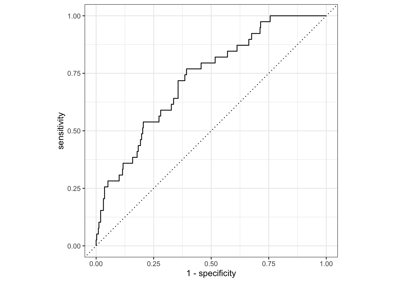
gender_many_prob |>
  roc_auc(
    truth = artist_gender,
    .pred_Female,
    event_level = "second"
  )
# A tibble: 1 × 3
.metric .estimator .estimate
<chr> <chr> <dbl>
1 roc_auc binary 0.727Add response here.
At the default prediction threshold of \(0.5\), the model is useless. It has a high accuracy, but this is due to the class imbalance in the data. However, the ROC curve and AUC show that the model can better balance the trade-off between sensitivity and specificity by adjusting the prediction threshold. The AUC is approximately \(0.72\) which is better than random guessing, though still with much room for improvement.
Adjust prediction threshold
Demo: Instead of attempting to fit a new model, let’s adjust the prediction threshold of the full model to see if we can improve its performance. Test several different prediction threshold values (e.g. any value between 0 and 1) and evaluate the model’s performance at each threshold. What are the trade-offs for different threshold values?
threshold_data <- threshold_perf(
  # data frame containing predicted probabilities
  .data = gender_many_prob,
  # true outcome
  truth = artist_gender,
  # predicted probability artist is female
  estimate = .pred_Female,
  # sequence of threshold values to test
  thresholds = seq(0, .5, by = 0.0025),
  # metrics to calculate
  metrics = multi_metric,
  # ensure "female" is treated as the event of interest
  event_level = "second"
)

ggplot(threshold_data, aes(x = .threshold, y = .estimate, color = .metric)) +
  geom_line() +
  theme_minimal() +
  scale_color_viridis_d(end = 0.9) +
  labs(
    x = "'Male' Threshold\n(above this value is predicted 'male')",
    y = "Metric Estimate",
    title = "Balancing performance by varying the threshold"
  )
Add response here.
As we decrease the threshold, the test set accuracy and sensitivity (probability that the model predicts “Male” given that the artist is actually male) decreases, but specificity (probability that the model predicts “Female” given that the artist is actually female) increases.
Session information
sessioninfo::session_info()─ Session info ───────────────────────────────────────────────────────────────
setting value
version R version 4.3.2 (2023-10-31)
os macOS Ventura 13.5.2
system aarch64, darwin20
ui X11
language (EN)
collate en_US.UTF-8
ctype en_US.UTF-8
tz America/New_York
date 2024-03-28
pandoc 3.1.1 @ /Applications/RStudio.app/Contents/Resources/app/quarto/bin/tools/ (via rmarkdown)
─ Packages ───────────────────────────────────────────────────────────────────
package * version date (UTC) lib source
arthistory * 0.1.0 2022-05-03 [1] CRAN (R 4.3.0)
backports 1.4.1 2021-12-13 [1] CRAN (R 4.3.0)
base64enc 0.1-3 2015-07-28 [1] CRAN (R 4.3.0)
broom * 1.0.5 2023-06-09 [1] CRAN (R 4.3.0)
class 7.3-22 2023-05-03 [1] CRAN (R 4.3.2)
cli 3.6.2 2023-12-11 [1] CRAN (R 4.3.1)
codetools 0.2-19 2023-02-01 [1] CRAN (R 4.3.2)
colorspace 2.1-0 2023-01-23 [1] CRAN (R 4.3.0)
data.table 1.14.10 2023-12-08 [1] CRAN (R 4.3.1)
dials * 1.2.0 2023-04-03 [1] CRAN (R 4.3.0)
DiceDesign 1.10 2023-12-07 [1] CRAN (R 4.3.1)
digest 0.6.34 2024-01-11 [1] CRAN (R 4.3.1)
dplyr * 1.1.4 2023-11-17 [1] CRAN (R 4.3.1)
evaluate 0.23 2023-11-01 [1] CRAN (R 4.3.1)
fansi 1.0.6 2023-12-08 [1] CRAN (R 4.3.1)
farver 2.1.1 2022-07-06 [1] CRAN (R 4.3.0)
fastmap 1.1.1 2023-02-24 [1] CRAN (R 4.3.0)
forcats * 1.0.0 2023-01-29 [1] CRAN (R 4.3.0)
foreach 1.5.2 2022-02-02 [1] CRAN (R 4.3.0)
furrr 0.3.1 2022-08-15 [1] CRAN (R 4.3.0)
future 1.33.1 2023-12-22 [1] CRAN (R 4.3.1)
future.apply 1.11.1 2023-12-21 [1] CRAN (R 4.3.1)
generics 0.1.3 2022-07-05 [1] CRAN (R 4.3.0)
ggplot2 * 3.4.4 2023-10-12 [1] CRAN (R 4.3.1)
globals 0.16.2 2022-11-21 [1] CRAN (R 4.3.0)
glue 1.7.0 2024-01-09 [1] CRAN (R 4.3.1)
gower 1.0.1 2022-12-22 [1] CRAN (R 4.3.0)
GPfit 1.0-8 2019-02-08 [1] CRAN (R 4.3.0)
gtable 0.3.4 2023-08-21 [1] CRAN (R 4.3.0)
hardhat 1.3.0 2023-03-30 [1] CRAN (R 4.3.0)
here 1.0.1 2020-12-13 [1] CRAN (R 4.3.0)
hms 1.1.3 2023-03-21 [1] CRAN (R 4.3.0)
htmltools 0.5.7 2023-11-03 [1] CRAN (R 4.3.1)
htmlwidgets 1.6.4 2023-12-06 [1] CRAN (R 4.3.1)
infer * 1.0.5 2023-09-06 [1] CRAN (R 4.3.0)
ipred 0.9-14 2023-03-09 [1] CRAN (R 4.3.0)
iterators 1.0.14 2022-02-05 [1] CRAN (R 4.3.0)
jsonlite 1.8.8 2023-12-04 [1] CRAN (R 4.3.1)
knitr 1.45 2023-10-30 [1] CRAN (R 4.3.1)
labeling 0.4.3 2023-08-29 [1] CRAN (R 4.3.0)
lattice 0.21-9 2023-10-01 [1] CRAN (R 4.3.2)
lava 1.7.3 2023-11-04 [1] CRAN (R 4.3.1)
lhs 1.1.6 2022-12-17 [1] CRAN (R 4.3.0)
lifecycle 1.0.4 2023-11-07 [1] CRAN (R 4.3.1)
listenv 0.9.0 2022-12-16 [1] CRAN (R 4.3.0)
lubridate * 1.9.3 2023-09-27 [1] CRAN (R 4.3.1)
magrittr 2.0.3 2022-03-30 [1] CRAN (R 4.3.0)
MASS 7.3-60 2023-05-04 [1] CRAN (R 4.3.2)
Matrix 1.6-1.1 2023-09-18 [1] CRAN (R 4.3.2)
modeldata * 1.2.0 2023-08-09 [1] CRAN (R 4.3.0)
munsell 0.5.0 2018-06-12 [1] CRAN (R 4.3.0)
nnet 7.3-19 2023-05-03 [1] CRAN (R 4.3.2)
parallelly 1.36.0 2023-05-26 [1] CRAN (R 4.3.0)
parsnip * 1.2.0 2024-02-16 [1] CRAN (R 4.3.1)
pillar 1.9.0 2023-03-22 [1] CRAN (R 4.3.0)
pkgconfig 2.0.3 2019-09-22 [1] CRAN (R 4.3.0)
probably * 1.0.3 2024-02-23 [1] CRAN (R 4.3.1)
prodlim 2023.08.28 2023-08-28 [1] CRAN (R 4.3.0)
purrr * 1.0.2 2023-08-10 [1] CRAN (R 4.3.0)
R6 2.5.1 2021-08-19 [1] CRAN (R 4.3.0)
Rcpp 1.0.12 2024-01-09 [1] CRAN (R 4.3.1)
readr * 2.1.5 2024-01-10 [1] CRAN (R 4.3.1)
recipes * 1.0.9 2023-12-13 [1] CRAN (R 4.3.1)
repr 1.1.6 2023-01-26 [1] CRAN (R 4.3.0)
rlang 1.1.3 2024-01-10 [1] CRAN (R 4.3.1)
rmarkdown 2.25 2023-09-18 [1] CRAN (R 4.3.1)
rpart 4.1.21 2023-10-09 [1] CRAN (R 4.3.2)
rprojroot 2.0.4 2023-11-05 [1] CRAN (R 4.3.1)
rsample * 1.2.0 2023-08-23 [1] CRAN (R 4.3.0)
rstudioapi 0.15.0 2023-07-07 [1] CRAN (R 4.3.0)
scales * 1.2.1 2024-01-18 [1] Github (r-lib/scales@c8eb772)
sessioninfo 1.2.2 2021-12-06 [1] CRAN (R 4.3.0)
skimr * 2.1.5 2022-12-23 [1] CRAN (R 4.3.0)
stringi 1.8.3 2023-12-11 [1] CRAN (R 4.3.1)
stringr * 1.5.1 2023-11-14 [1] CRAN (R 4.3.1)
survival 3.5-7 2023-08-14 [1] CRAN (R 4.3.2)
tibble * 3.2.1 2023-03-20 [1] CRAN (R 4.3.0)
tidymodels * 1.1.1 2023-08-24 [1] CRAN (R 4.3.0)
tidyr * 1.3.0 2023-01-24 [1] CRAN (R 4.3.0)
tidyselect 1.2.0 2022-10-10 [1] CRAN (R 4.3.0)
tidyverse * 2.0.0 2023-02-22 [1] CRAN (R 4.3.0)
timechange 0.2.0 2023-01-11 [1] CRAN (R 4.3.0)
timeDate 4032.109 2023-12-14 [1] CRAN (R 4.3.1)
tune * 1.1.2 2023-08-23 [1] CRAN (R 4.3.0)
tzdb 0.4.0 2023-05-12 [1] CRAN (R 4.3.0)
utf8 1.2.4 2023-10-22 [1] CRAN (R 4.3.1)
vctrs 0.6.5 2023-12-01 [1] CRAN (R 4.3.1)
viridisLite 0.4.2 2023-05-02 [1] CRAN (R 4.3.0)
withr 2.5.2 2023-10-30 [1] CRAN (R 4.3.1)
workflows * 1.1.4 2024-02-19 [1] CRAN (R 4.3.1)
workflowsets * 1.0.1 2023-04-06 [1] CRAN (R 4.3.0)
xfun 0.41 2023-11-01 [1] CRAN (R 4.3.1)
yaml 2.3.8 2023-12-11 [1] CRAN (R 4.3.1)
yardstick * 1.3.0 2024-01-19 [1] CRAN (R 4.3.1)
[1] /Library/Frameworks/R.framework/Versions/4.3-arm64/Resources/library
──────────────────────────────────────────────────────────────────────────────Footnotes
Courtesy of #TidyTuesday↩︎