library(tidyverse)
library(tidymodels)
library(skimr)

chipotle <- read_csv(file = "data/chipotle.csv")Do you get more food when you order in-person at Chipotle?
Suggested answers
Application exercise
Answers
Inspired by this Reddit post, we will conduct a hypothesis test to determine if there is a difference in the weight of Chipotle orders between in-person and online orders. The data was originally collected by Zackary Smigel, and a cleaned copy be found in data/chipotle.csv.
Throughout the application exercise we will use the infer package which is part of tidymodels to conduct our permutation tests.
skim(chipotle)| Name | chipotle |
| Number of rows | 30 |
| Number of columns | 7 |
| _______________________ | |
| Column type frequency: | |
| character | 4 |
| Date | 1 |
| numeric | 2 |
| ________________________ | |
| Group variables | None |
Variable type: character
| skim_variable | n_missing | complete_rate | min | max | empty | n_unique | whitespace |
|---|---|---|---|---|---|---|---|
| order | 0 | 1 | 6 | 6 | 0 | 2 | 0 |
| meat | 0 | 1 | 7 | 8 | 0 | 2 | 0 |
| store | 0 | 1 | 7 | 7 | 0 | 3 | 0 |
| food | 0 | 1 | 4 | 7 | 0 | 2 | 0 |
Variable type: Date
| skim_variable | n_missing | complete_rate | min | max | median | n_unique |
|---|---|---|---|---|---|---|
| date | 0 | 1 | 2024-01-12 | 2024-02-10 | 2024-01-26 | 30 |
Variable type: numeric
| skim_variable | n_missing | complete_rate | mean | sd | p0 | p25 | p50 | p75 | p100 | hist |
|---|---|---|---|---|---|---|---|---|---|---|
| day | 0 | 1 | 15.5 | 8.80 | 1.00 | 8.25 | 15.50 | 22.75 | 30.00 | ▇▇▇▇▇ |
| weight | 0 | 1 | 810.8 | 123.37 | 510.29 | 715.82 | 793.79 | 907.18 | 1048.93 | ▁▆▇▇▂ |
The variable we will use in this analysis is weight which records the total weight of the meal in grams.
Hypotheses
We wish to test the claim that the difference in weight between in-person and online orders must be due to something other than chance.
ggplot(data = chipotle, aes(x = weight, color = order)) +
  geom_density() +
  labs(
    title = "Chipotle Weight Distribution",
    x = "Weight (g)",
    y = "Count"
  )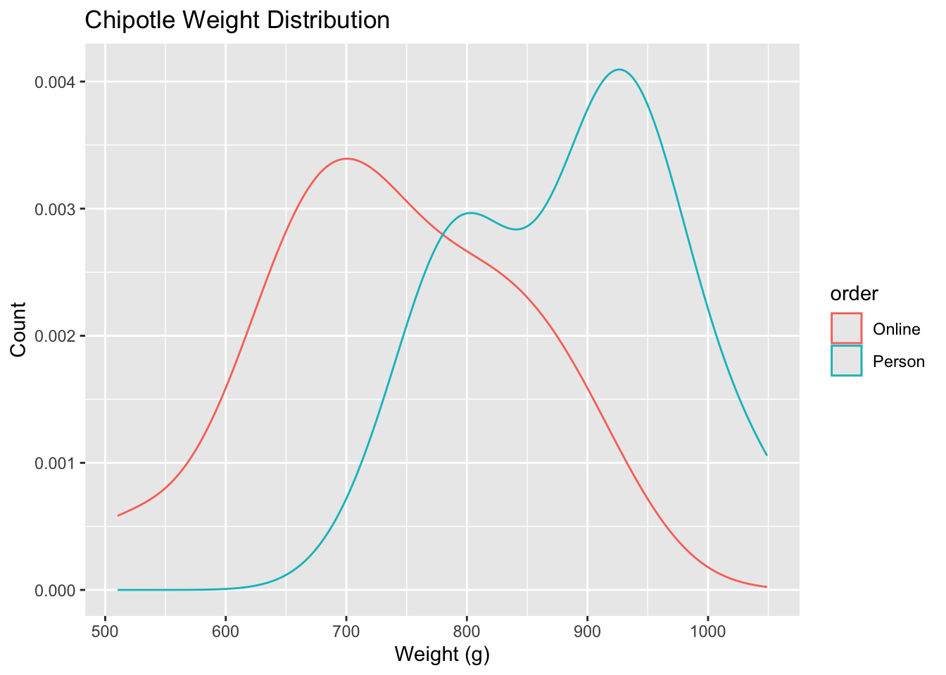
- Your turn: Write out the correct null and alternative hypothesis in terms of the difference in means between in-person and online orders. Do this in both words and in proper notation.
Null hypothesis: The difference in means between in-person and online Chipotle orders is \(0\).
\[H_0: \mu_{\text{in-person}} - \mu_{\text{online}} = 0\]
Alternative hypothesis: The difference in means between in-person and online Chipotle orders is not \(0\).
\[H_A: \mu_{\text{in-person}} - \mu_{\text{online}} \neq 0\]
Observed data
Our goal is to use the collected data and calculate the probability of a sample statistic at least as extreme as the one observed in our data if in fact the null hypothesis is true.
- Demo: Calculate and report the sample statistic below using proper notation.
chipotle |>
  group_by(order) |>
  summarize(mean_weight = mean(weight))
# A tibble: 2 × 2
order mean_weight
<chr> <dbl>
1 Online 735.
2 Person 886.\[\bar{x}_{\text{in-person}} - \bar{x}_{\text{online}} = 886 - 735 \approx 151\]
The null distribution
Let’s use permutation-based methods to conduct the hypothesis test specified above.
Generate
We’ll start by generating the null distribution.
- Demo: Generate the null distribution.
set.seed(123)null_dist <- chipotle |>
# specify the response and explanatory variable
specify(weight ~ order) |>
# declare the null hypothesis
hypothesize(null = "independence") |>
# simulate the null distribution
generate(reps = 1000, type = "permute") |>
# calculate the difference in means for each permutation
calculate(stat = "diff in means", order = c("Person", "Online"))- Your turn: Take a look at
null_dist. What does each element in this distribution represent?
null_distResponse: weight (numeric)
Explanatory: order (factor)
Null Hypothesis: independence
# A tibble: 1,000 × 2
replicate stat
<int> <dbl>
1 1 -68.0
2 2 37.8
3 3 15.1
4 4 -30.2
5 5 37.8
6 6 -3.78
7 7 -56.7
8 8 26.5
9 9 -37.8
10 10 45.4
# ℹ 990 more rowsAdd response here. Each element in this distribution represents the difference in means between in-person and online orders for each permutation.
Visualize
Question: Before you visualize the distribution of
null_dist– at what value would you expect this distribution to be centered? Why?Add response here. At 0, since we created this distribution assuming \(\mu_{\text{in-person}} - \mu_{\text{online}} = 0\).
Demo: Create an appropriate visualization for your null distribution. Does the center of the distribution match what you guessed in the previous question?
visualize(null_dist)
- Demo: Now, add a vertical red line on your null distribution that represents your sample statistic.
visualize(null_dist) +
  geom_vline(xintercept = 151, color = "red")
Question: Based on the position of this line, does your observed sample difference in means appear to be an unusual observation under the assumption of the null hypothesis?
Add response here. Yes, it is far and to the right.
p-value
Above, we eyeballed how likely/unlikely our observed mean is. Now, let’s actually quantify it using a p-value.
Question: What is a p-value?
Add response here. The probability of the observed sample statistic, or something more extreme in the direction of the alternative hypothesis, if in fact the null hypothesis is true.
Guesstimate the p-value
- Demo: Visualize the p-value.
visualize(null_dist) +
  geom_vline(xintercept = 151, color = "red") +
  geom_vline(xintercept = -151, color = "red", linetype = "dashed")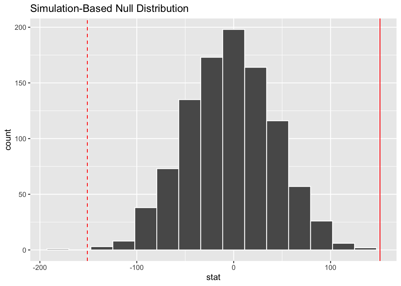
Your turn: What is you guesstimate of the p-value?
Add response here. Pretty small, maybe \(0.02\)?
Calculate the p-value
# calculate sample statistic
d_hat <- chipotle |>
  specify(weight ~ order) |>
  # calculate the observed difference in means
  calculate(stat = "diff in means", order = c("Person", "Online"))

# visualize simulated p-value
visualize(null_dist) +
  shade_p_value(obs_stat = d_hat, direction = "two-sided")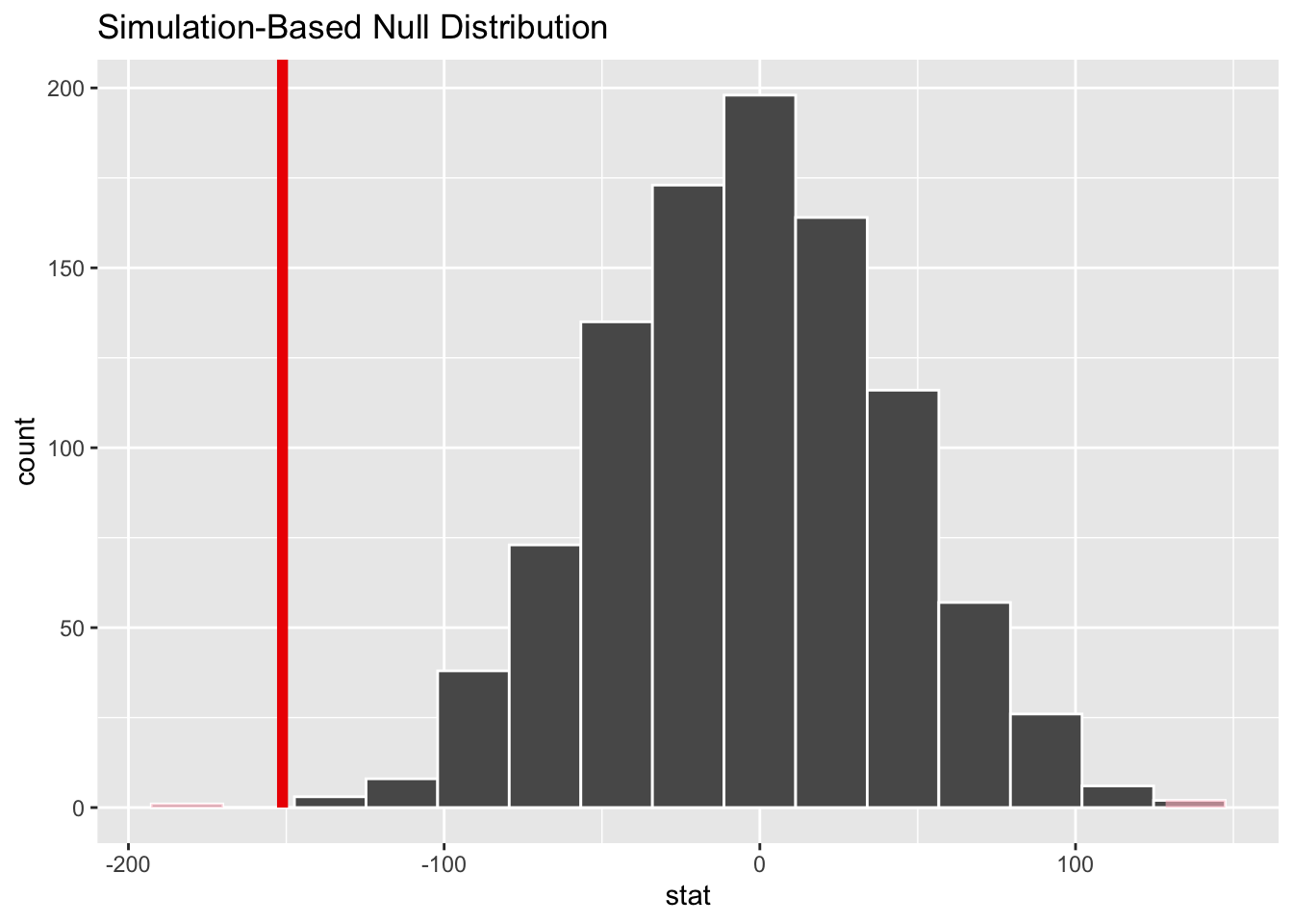
# calculate simulated p-value
null_dist |>
  get_p_value(obs_stat = d_hat, direction = "two-sided")
# A tibble: 1 × 1
p_value
<dbl>
1 0.002Conclusion
Your turn: What is the conclusion of the hypothesis test based on the p-value you calculated? Make sure to frame it in context of the data and the research question. Use a significance level of 5% to make your conclusion.
Add response here. Since the p-value is smaller than the significance level, we reject the null hypothesis. The data provides convincing evidence that the difference in weight between online and in-person Chipotle orders is different from 0.
Demo: Interpret the p-value in context of the data and the research question.
Add response here. If in fact the true difference in means between the weight of online and in-person Chipotle orders is 0, the probability of observing a sample of 30 orders where the difference in means is 151 grams or higher, or -151 grams or lower, is approximately 0.002.
Reframe as a linear regression model
While we originally evaluated the null/alternative hypotheses as a difference in means, we could also frame this as a regression problem where the outcome of interest (weight of the order) is a continuous variable. Framing it this way allows us to include additional explanatory variables in our model which may account for some of the variation in weight.
Single explanatory variable
Demo: Let’s reevaluate the original hypotheses using a linear regression model. Notice the similarities and differences in the code compared to a difference in means, and that the obtained p-value should be nearly identical to the results from the difference in means test.
# observed fit
obs_fit <- chipotle |>
  # specify the response and explanatory variable
  specify(weight ~ order) |>
  # fit the linear regression model
  fit()

# null distribution
set.seed(123)

null_dist <- chipotle |>
  # specify the response and explanatory variable
  specify(weight ~ order) |>
  # declare the null hypothesis
  hypothesize(null = "independence") |>
  # simulate the null distribution
  generate(reps = 1000, type = "permute") |>
  # estimate the linear regression model for each permutation
  fit()

# examine p-value
visualize(null_dist) +
  shade_p_value(obs_stat = obs_fit, direction = "two-sided")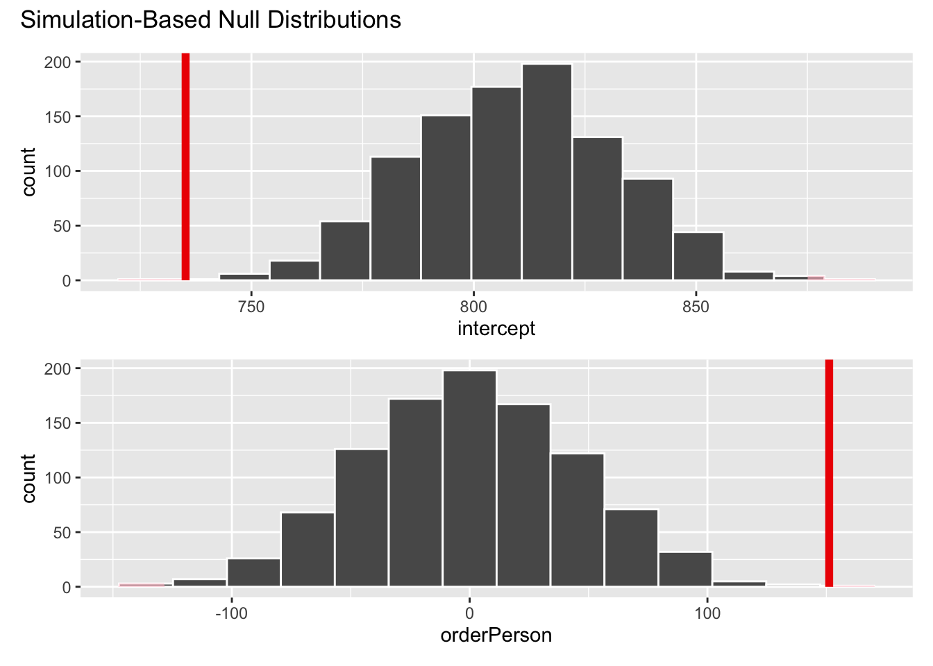
# calculate p-value
null_dist |>
  get_p_value(obs_stat = obs_fit, direction = "two-sided")
# A tibble: 2 × 2
term p_value
<chr> <dbl>
1 intercept 0.002
2 orderPerson 0.002Multiple explanatory variables
Demo: Now let’s also account for additional variables that likely influence the weight of the order.
- Protein type (
meat) - Type of meal (
food) - burrito or bowl - Store (
store) - at which Chipotle location the order was placed
# observed results
obs_fit <- chipotle |>
  specify(weight ~ order + meat + food + store) |>
  fit()

# permutation null distribution
null_dist <- chipotle |>
  specify(weight ~ order + meat + food + store) |>
  hypothesize(null = "independence") |>
  generate(reps = 10000, type = "permute") |>
  fit()

# examine p-value
visualize(null_dist) +
  shade_p_value(obs_stat = obs_fit, direction = "two-sided")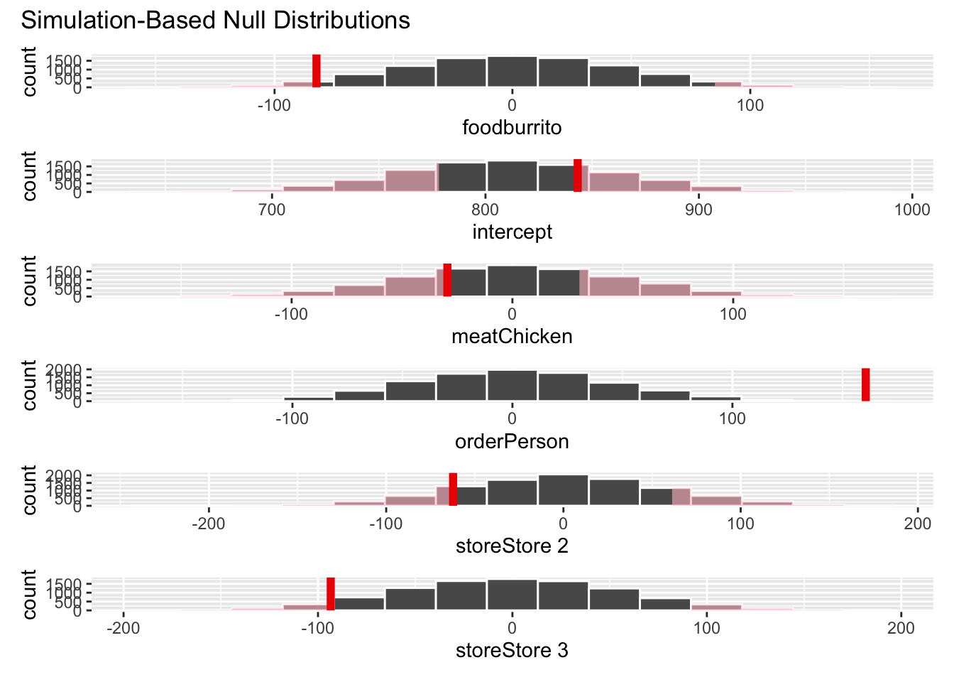
null_dist |>
  get_p_value(obs_stat = obs_fit, direction = "two-sided")
# A tibble: 6 × 2
term p_value
<chr> <dbl>
1 foodburrito 0.0628
2 intercept 0.524
3 meatChicken 0.546
4 orderPerson 0.0002
5 storeStore 2 0.272
6 storeStore 3 0.0938Your turn: What is the conclusion of the hypothesis test based on the p-value you calculated? Make sure to frame it in context of the data and the research question. Use a significance level of 5% to make your conclusion.
Add response here. Since the p-value is smaller than the significance level, we reject the null hypothesis. The data provides convincing evidence that the difference in weight between online and in-person Chipotle orders is different from 0, holding constant the meat, meal type, and store location.
Your turn: Interpret the p-value for the order in context of the data and the research question.
Add response here. If in fact the true difference in means between the weight of online and in-person Chipotle orders is 0, the probability of observing a sample of 30 orders where the difference in means is 151 grams or higher, or -151 grams or lower, is approximately 0.
Compare to CLT-based method
Demo: Let’s compare the p-value obtained from the permutation test to the p-value obtained from that derived using the Central Limit Theorem (CLT).
linear_reg() |>
  fit(weight ~ order + meat + food + store, data = chipotle) |>
  tidy()
# A tibble: 6 × 5
term estimate std.error statistic p.value
<chr> <dbl> <dbl> <dbl> <dbl>
1 (Intercept) 843. 36.4 23.2 6.30e-18
2 orderPerson 161. 30.2 5.31 1.88e- 5
3 meatChicken -29.5 32.5 -0.907 3.73e- 1
4 foodburrito -82.4 30.2 -2.73 1.18e- 2
5 storeStore 2 -62.3 36.7 -1.69 1.03e- 1
6 storeStore 3 -93.4 36.7 -2.54 1.78e- 2Your turn: What is the p-value obtained from the CLT-based method? How does it compare to the p-value obtained from the permutation test?
Add response here. The p-value obtained from the CLT-based method is approximately \(0.00001\), which is smaller than the p-value obtained from the permutation test. This is likely due to the permutation test being more robust to violations of the assumptions of the CLT (in this case, sample size).
Session information
sessioninfo::session_info()─ Session info ───────────────────────────────────────────────────────────────
setting value
version R version 4.3.2 (2023-10-31)
os macOS Ventura 13.6.6
system aarch64, darwin20
ui X11
language (EN)
collate en_US.UTF-8
ctype en_US.UTF-8
tz America/New_York
date 2024-04-25
pandoc 3.1.1 @ /Applications/RStudio.app/Contents/Resources/app/quarto/bin/tools/ (via rmarkdown)
─ Packages ───────────────────────────────────────────────────────────────────
package * version date (UTC) lib source
archive 1.1.7 2023-12-11 [1] CRAN (R 4.3.1)
backports 1.4.1 2021-12-13 [1] CRAN (R 4.3.0)
base64enc 0.1-3 2015-07-28 [1] CRAN (R 4.3.0)
bit 4.0.5 2022-11-15 [1] CRAN (R 4.3.0)
bit64 4.0.5 2020-08-30 [1] CRAN (R 4.3.0)
broom * 1.0.5 2023-06-09 [1] CRAN (R 4.3.0)
class 7.3-22 2023-05-03 [1] CRAN (R 4.3.2)
cli 3.6.2 2023-12-11 [1] CRAN (R 4.3.1)
codetools 0.2-19 2023-02-01 [1] CRAN (R 4.3.2)
colorspace 2.1-0 2023-01-23 [1] CRAN (R 4.3.0)
crayon 1.5.2 2022-09-29 [1] CRAN (R 4.3.0)
data.table 1.15.4 2024-03-30 [1] CRAN (R 4.3.1)
dials * 1.2.1 2024-02-22 [1] CRAN (R 4.3.1)
DiceDesign 1.10 2023-12-07 [1] CRAN (R 4.3.1)
digest 0.6.35 2024-03-11 [1] CRAN (R 4.3.1)
dplyr * 1.1.4 2023-11-17 [1] CRAN (R 4.3.1)
evaluate 0.23 2023-11-01 [1] CRAN (R 4.3.1)
fansi 1.0.6 2023-12-08 [1] CRAN (R 4.3.1)
farver 2.1.1 2022-07-06 [1] CRAN (R 4.3.0)
fastmap 1.1.1 2023-02-24 [1] CRAN (R 4.3.0)
forcats * 1.0.0 2023-01-29 [1] CRAN (R 4.3.0)
foreach 1.5.2 2022-02-02 [1] CRAN (R 4.3.0)
furrr 0.3.1 2022-08-15 [1] CRAN (R 4.3.0)
future 1.33.2 2024-03-26 [1] CRAN (R 4.3.1)
future.apply 1.11.2 2024-03-28 [1] CRAN (R 4.3.1)
generics 0.1.3 2022-07-05 [1] CRAN (R 4.3.0)
ggplot2 * 3.5.1 2024-04-23 [1] CRAN (R 4.3.1)
globals 0.16.3 2024-03-08 [1] CRAN (R 4.3.1)
glue 1.7.0 2024-01-09 [1] CRAN (R 4.3.1)
gower 1.0.1 2022-12-22 [1] CRAN (R 4.3.0)
GPfit 1.0-8 2019-02-08 [1] CRAN (R 4.3.0)
gtable 0.3.5 2024-04-22 [1] CRAN (R 4.3.1)
hardhat 1.3.1 2024-02-02 [1] CRAN (R 4.3.1)
here 1.0.1 2020-12-13 [1] CRAN (R 4.3.0)
hms 1.1.3 2023-03-21 [1] CRAN (R 4.3.0)
htmltools 0.5.8.1 2024-04-04 [1] CRAN (R 4.3.1)
htmlwidgets 1.6.4 2023-12-06 [1] CRAN (R 4.3.1)
infer * 1.0.7 2024-03-25 [1] CRAN (R 4.3.1)
ipred 0.9-14 2023-03-09 [1] CRAN (R 4.3.0)
iterators 1.0.14 2022-02-05 [1] CRAN (R 4.3.0)
jsonlite 1.8.8 2023-12-04 [1] CRAN (R 4.3.1)
knitr 1.45 2023-10-30 [1] CRAN (R 4.3.1)
labeling 0.4.3 2023-08-29 [1] CRAN (R 4.3.0)
lattice 0.21-9 2023-10-01 [1] CRAN (R 4.3.2)
lava 1.8.0 2024-03-05 [1] CRAN (R 4.3.1)
lhs 1.1.6 2022-12-17 [1] CRAN (R 4.3.0)
lifecycle 1.0.4 2023-11-07 [1] CRAN (R 4.3.1)
listenv 0.9.1 2024-01-29 [1] CRAN (R 4.3.1)
lubridate * 1.9.3 2023-09-27 [1] CRAN (R 4.3.1)
magrittr 2.0.3 2022-03-30 [1] CRAN (R 4.3.0)
MASS 7.3-60 2023-05-04 [1] CRAN (R 4.3.2)
Matrix 1.6-1.1 2023-09-18 [1] CRAN (R 4.3.2)
modeldata * 1.3.0 2024-01-21 [1] CRAN (R 4.3.1)
munsell 0.5.1 2024-04-01 [1] CRAN (R 4.3.1)
nnet 7.3-19 2023-05-03 [1] CRAN (R 4.3.2)
parallelly 1.37.1 2024-02-29 [1] CRAN (R 4.3.1)
parsnip * 1.2.1 2024-03-22 [1] CRAN (R 4.3.1)
patchwork 1.2.0 2024-01-08 [1] CRAN (R 4.3.1)
pillar 1.9.0 2023-03-22 [1] CRAN (R 4.3.0)
pkgconfig 2.0.3 2019-09-22 [1] CRAN (R 4.3.0)
prodlim 2023.08.28 2023-08-28 [1] CRAN (R 4.3.0)
purrr * 1.0.2 2023-08-10 [1] CRAN (R 4.3.0)
R6 2.5.1 2021-08-19 [1] CRAN (R 4.3.0)
Rcpp 1.0.12 2024-01-09 [1] CRAN (R 4.3.1)
readr * 2.1.5 2024-01-10 [1] CRAN (R 4.3.1)
recipes * 1.0.10 2024-02-18 [1] CRAN (R 4.3.1)
repr 1.1.6 2023-01-26 [1] CRAN (R 4.3.0)
rlang 1.1.3 2024-01-10 [1] CRAN (R 4.3.1)
rmarkdown 2.26 2024-03-05 [1] CRAN (R 4.3.1)
rpart 4.1.21 2023-10-09 [1] CRAN (R 4.3.2)
rprojroot 2.0.4 2023-11-05 [1] CRAN (R 4.3.1)
rsample * 1.2.1 2024-03-25 [1] CRAN (R 4.3.1)
rstudioapi 0.16.0 2024-03-24 [1] CRAN (R 4.3.1)
scales * 1.3.0 2023-11-28 [1] CRAN (R 4.3.1)
sessioninfo 1.2.2 2021-12-06 [1] CRAN (R 4.3.0)
skimr * 2.1.5 2022-12-23 [1] CRAN (R 4.3.0)
stringi 1.8.3 2023-12-11 [1] CRAN (R 4.3.1)
stringr * 1.5.1 2023-11-14 [1] CRAN (R 4.3.1)
survival 3.5-7 2023-08-14 [1] CRAN (R 4.3.2)
tibble * 3.2.1 2023-03-20 [1] CRAN (R 4.3.0)
tidymodels * 1.2.0 2024-03-25 [1] CRAN (R 4.3.1)
tidyr * 1.3.1 2024-01-24 [1] CRAN (R 4.3.1)
tidyselect 1.2.1 2024-03-11 [1] CRAN (R 4.3.1)
tidyverse * 2.0.0 2023-02-22 [1] CRAN (R 4.3.0)
timechange 0.3.0 2024-01-18 [1] CRAN (R 4.3.1)
timeDate 4032.109 2023-12-14 [1] CRAN (R 4.3.1)
tune * 1.2.1 2024-04-18 [1] CRAN (R 4.3.1)
tzdb 0.4.0 2023-05-12 [1] CRAN (R 4.3.0)
utf8 1.2.4 2023-10-22 [1] CRAN (R 4.3.1)
vctrs 0.6.5 2023-12-01 [1] CRAN (R 4.3.1)
vroom 1.6.5 2023-12-05 [1] CRAN (R 4.3.1)
withr 3.0.0 2024-01-16 [1] CRAN (R 4.3.1)
workflows * 1.1.4 2024-02-19 [1] CRAN (R 4.3.1)
workflowsets * 1.1.0 2024-03-21 [1] CRAN (R 4.3.1)
xfun 0.43 2024-03-25 [1] CRAN (R 4.3.1)
yaml 2.3.8 2023-12-11 [1] CRAN (R 4.3.1)
yardstick * 1.3.1 2024-03-21 [1] CRAN (R 4.3.1)
[1] /Library/Frameworks/R.framework/Versions/4.3-arm64/Resources/library
──────────────────────────────────────────────────────────────────────────────