library(tidyverse)
library(tidymodels)
library(unvotes)
library(themis)
library(discrim)
library(tidytext)
library(embed)

theme_set(theme_minimal())

set.seed(123)Dimensionality reduction of UN voting patterns
Suggested answers
Application exercise
Answers
How do various countries vote in the United Nations General Assembly? Can we use roll call votes to locate countries along meaningful dimensions? Can we use those dimensions to predict future voting behavior?
In this application exercise we will use unsupervised learning and dimension reduction techniques to explore the voting patterns of countries in the United Nations General Assembly. We will use the un_votes dataset from the unvotes package,1 which contains information on roll call votes in the United Nations General Assembly from 1946 to 2016. We will use principal components analysis (PCA) to reduce the dimensionality of the data and explore the voting patterns of countries. Then we will attempt to fit a supervised classification model to predict future roll call votes using first few principal components.
# load data frames from unvotes package
data("un_votes")
data("un_roll_call_issues")

# convert to tibbles
unvotes <- un_votes |>
  as_tibble()

issues <- un_roll_call_issues |>
  as_tibble()

# restructure roll-call votes as one column for each vote
unvotes_df <- unvotes |>
  select(country, rcid, vote) |>
  mutate(
    vote = factor(vote, levels = c("no", "abstain", "yes")),
    vote = as.numeric(vote),
    rcid = paste0("rcid_", rcid)
  ) |>
  pivot_wider(names_from = "rcid", values_from = "vote", values_fill = 2)
unvotes_df
# A tibble: 200 × 6,465
country rcid_3 rcid_4 rcid_5 rcid_6 rcid_7 rcid_8 rcid_9 rcid_10 rcid_11
<chr> <dbl> <dbl> <dbl> <dbl> <dbl> <dbl> <dbl> <dbl> <dbl>
1 United Stat… 3 1 1 1 1 1 3 3 3
2 Canada 1 1 1 1 1 3 3 3 3
3 Cuba 3 1 3 3 3 3 3 3 3
4 Haiti 3 1 1 2 3 2 3 3 2
5 Dominican R… 3 1 1 2 3 3 3 3 3
6 Mexico 3 1 3 3 3 3 3 3 2
7 Guatemala 3 1 1 1 2 3 2 3 2
8 Honduras 3 1 3 3 3 2 2 2 3
9 El Salvador 3 1 3 2 2 2 3 1 2
10 Nicaragua 3 1 3 3 3 2 2 1 2
# ℹ 190 more rows
# ℹ 6,455 more variables: rcid_12 <dbl>, rcid_13 <dbl>, rcid_14 <dbl>,
# rcid_15 <dbl>, rcid_16 <dbl>, rcid_17 <dbl>, rcid_18 <dbl>, rcid_19 <dbl>,
# rcid_20 <dbl>, rcid_21 <dbl>, rcid_22 <dbl>, rcid_23 <dbl>, rcid_24 <dbl>,
# rcid_25 <dbl>, rcid_26 <dbl>, rcid_27 <dbl>, rcid_28 <dbl>, rcid_29 <dbl>,
# rcid_30 <dbl>, rcid_31 <dbl>, rcid_32 <dbl>, rcid_33 <dbl>, rcid_34 <dbl>,
# rcid_35 <dbl>, rcid_36 <dbl>, rcid_37 <dbl>, rcid_38 <dbl>, …- Each “rcid” is a different vote in the General Assembly
- Countries can vote either Yes (3), Abstain (2), or No (1)
Principal components analysis
Define feature engineering recipe
Demo: Create a feature engineering recipe to normalize the votes and convert them to principal components.
pca_rec <- recipe(~ ., data = unvotes_df) |>
  # ignore the country column
  update_role(country, new_role = "id") |>
  # normalize the votes
  step_normalize(all_predictors()) |>
  # convert to principal components
  step_pca(all_predictors(), num_comp = 5)
pca_rec
Prep and bake the recipe
Demo: In order to use the recipe to transform the data, we need to prep() and bake() it. Notice this does not use the usual tidymodels workflow since there is no outcome to predict.
prep(recipe, training)fits the recipe to the training setbake(recipe, new_data)applies the recipe operations tonew_data
Tip
Manually prepping and baking the recipe can be helpful when troubleshooting supervised learning models if you are unsure exactly how the recipe is transforming the training data.
pca_prep <- prep(pca_rec)
pca_prep

bake(pca_prep, new_data = NULL)
# A tibble: 200 × 6
country PC1 PC2 PC3 PC4 PC5
<fct> <dbl> <dbl> <dbl> <dbl> <dbl>
1 United States -136. -13.8 -92.2 35.0 3.40
2 Canada -51.3 -65.6 -30.8 6.13 -10.3
3 Cuba 43.2 19.9 -0.309 -7.54 37.8
4 Haiti 20.8 -13.0 -8.30 19.7 11.4
5 Dominican Republic 21.0 -23.5 -7.70 30.5 6.93
6 Mexico 43.0 -23.6 -5.93 6.75 18.8
7 Guatemala 18.6 -23.6 -3.77 23.2 12.5
8 Honduras 22.0 -27.2 -9.10 29.4 6.44
9 El Salvador 23.1 -23.0 -2.02 27.4 15.7
10 Nicaragua 29.5 -17.4 -2.15 29.8 13.2
# ℹ 190 more rowsExamine first two principal components
Your turn: Use the baked recipe to transform the data and visualize the first two principal components using a scatterplot. Label the countries as best you can. What patterns do you see?
bake(pca_prep, new_data = NULL) |>
  ggplot(mapping = aes(x = PC1, PC2, label = country)) +
  geom_point(alpha = 0.3, size = 2) +
  geom_text(check_overlap = TRUE, hjust = "inward")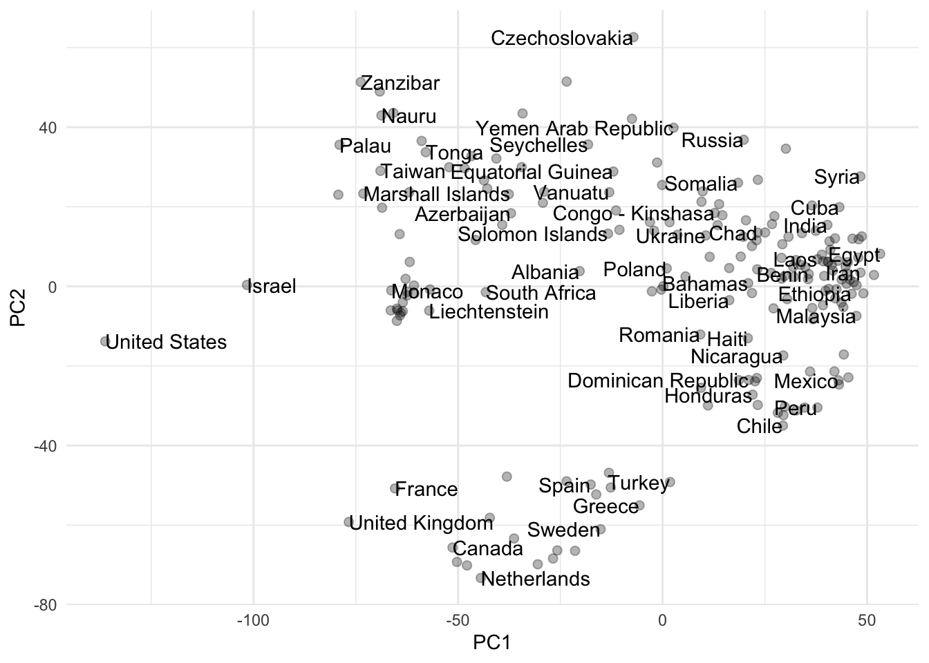
Add response here. Various interpretations possible. The United States and Israel seem to be separated from the rest of the countries, especially on the first dimension. Western European countries also seem to be clustered near each other on the first and second dimensions.
Which issues contribute to each principal component?
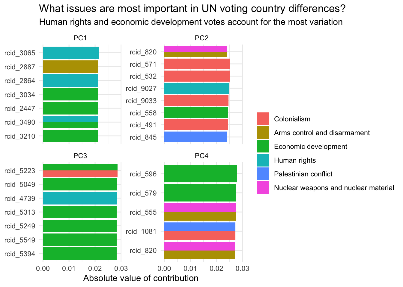
Demo: We can use the results from PCA to determine which specific votes load most strongly on to the first two dimensions.
# extract component scores for each roll call vote
pca_comps <- tidy(pca_prep, number = 2, type = "coef") |>
  # keep only the first 4 components
  filter(component %in% str_c("PC", 1:4)) |>
  # join to get issue names
  left_join(issues |>
              mutate(terms = str_c("rcid_", rcid))) |>
  filter(!is.na(issue))

# keep the top 8 roll call votes per component
pca_comps |>
  slice_max(order_by = abs(value), n = 8, by = component) |>
  # visualize absolute values
  mutate(value = abs(value),
         terms = fct_reorder(.f = terms, .x = value)) |>
  ggplot(mapping = aes(x = value, y = terms, fill = issue)) +
  geom_col(position = "dodge") +
  facet_wrap(facets = vars(component), scales = "free_y") +
  labs(
    x = "Absolute value of contribution",
    y = NULL, fill = NULL,
    title = "What issues are most important in UN voting country differences?",
    subtitle = "Human rights and economic development votes account for the most variation"
  )
Your turn: Visualize each roll call vote on the first vs. second principal components, faceting for each issue. What patterns, if any, emerge? Do the first two principal components seem to capture the issue-related variation in the data?
pca_comps |>
  # convert component scores to wide format - one column per principal component
  pivot_wider(
    names_from = component,
    values_from = value
  ) |>
  # pc1 vs. pc2
  ggplot(mapping = aes(x = PC1, y = PC2, color = issue)) +
  geom_point(alpha = 0.3) +
  scale_color_viridis_d(end = 0.8, guide = "none") +
  facet_wrap(facets = vars(issue))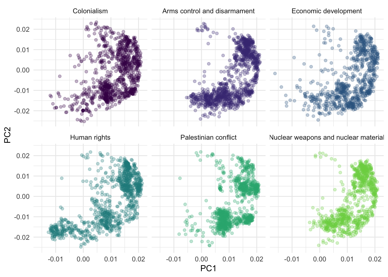
Add response here. They all seem to have a crescent shape. Nothing clearly distinguishing the issues on the first two dimensions. Might need to incorporate additional dimensions.
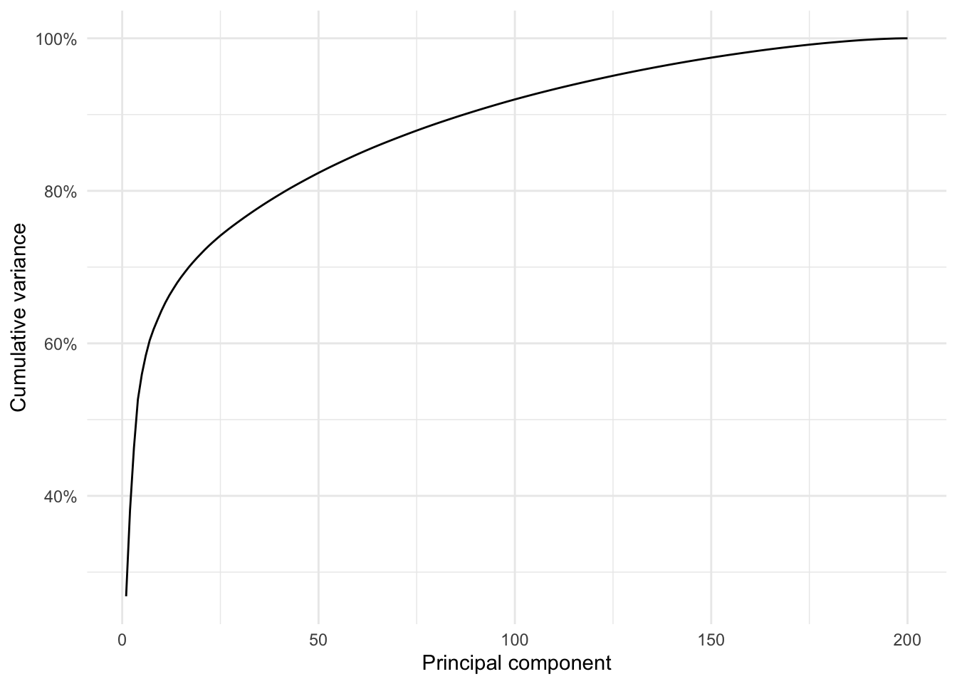
Variance explained
Demo: We can also visualize the percent variance explained by each principal component.
tidy(pca_prep, number = 2, type = "variance") |>
  filter(terms == "percent variance") |>
  ggplot(mapping = aes(x = component, y = value)) +
  geom_line() +
  scale_y_continuous(labels = label_percent(scale = 1)) +
  labs(
    x = "Principal component",
    y = "Percent variance"
  )
tidy(pca_prep, number = 2, type = "variance") |>
  filter(terms == "cumulative percent variance") |>
  ggplot(mapping = aes(x = component, y = value)) +
  geom_line() +
  scale_y_continuous(labels = label_percent(scale = 1)) +
  labs(
    x = "Principal component",
    y = "Cumulative variance"
  )
UMAP
Your turn: Instead of PCA, use UMAP to project the roll-call votes on to a non-linear, low-dimensional representation. What patterns do you see?
# recipe to generate umap dimensions
umap_rec <- recipe(~., data = unvotes_df) |>
  update_role(country, new_role = "id") |>
  step_normalize(all_predictors()) |>
  step_umap(all_predictors())

# prep the recipe
umap_prep <- prep(umap_rec)

# visualize the umap dimensions by country
bake(umap_prep, new_data = NULL) |>
  ggplot(mapping = aes(x = UMAP1, y = UMAP2, label = country)) +
  geom_point(alpha = 0.3, size = 2) +
  geom_text(check_overlap = TRUE, hjust = "inward")
Add response here. The UMAP plot shows a more complex structure than the PCA plot. There are four distinct clusters of countries along the two dimensions. The United States appears most similar to countries like South Africa, Armenia, and Liechtenstein.
Use PCA for predictive modeling
Combine UN vote data frames
# combine all relevant data frames
unvotes_mod_df <- unvotes |>
  left_join(y = un_roll_calls) |>
  left_join(y = un_roll_call_issues, relationship = "many-to-many") |>
  drop_na(issue) |>
  # eliminate duplicate observations
  distinct(country, rcid, vote, .keep_all = TRUE) |>
  select(rcid:vote, date, importantvote, issue)
unvotes_mod_df
# A tibble: 629,954 × 7
rcid country country_code vote date importantvote issue
<int> <chr> <chr> <fct> <date> <int> <fct>
1 6 United States US no 1946-01-04 0 Human…
2 6 Canada CA no 1946-01-04 0 Human…
3 6 Cuba CU yes 1946-01-04 0 Human…
4 6 Dominican Republic DO abstain 1946-01-04 0 Human…
5 6 Mexico MX yes 1946-01-04 0 Human…
6 6 Guatemala GT no 1946-01-04 0 Human…
7 6 Honduras HN yes 1946-01-04 0 Human…
8 6 El Salvador SV abstain 1946-01-04 0 Human…
9 6 Nicaragua NI yes 1946-01-04 0 Human…
10 6 Panama PA abstain 1946-01-04 0 Human…
# ℹ 629,944 more rowsSplit into training/test sets
unvotes_train <- unvotes_mod_df |>
  filter(year(date) < 2018)
unvotes_test <- unvotes_mod_df |>
  filter(year(date) >= 2018)
Generate PCA components using the training set
# convert to wide format, one column for each vote
unvotes_train_wide <- unvotes_train |>
  select(country, rcid, vote) |>
  mutate(
    vote = factor(vote, levels = c("no", "abstain", "yes")),
    vote = as.numeric(vote),
    rcid = str_c("rcid_", rcid)
  ) |>
  pivot_wider(names_from = "rcid", values_from = "vote", values_fill = 2)

# generate PCA scores and extract to data frame
pca_vals <- recipe(~ ., data = unvotes_train_wide) |>
  update_role(country, new_role = "id") |>
  step_normalize(all_predictors()) |>
  step_pca(all_predictors(), num_comp = 5) |>
  prep() |>
  bake(new_data = NULL)
Combine PCA components with vote-level training set
# define PCA recipe
unvotes_train <- unvotes_mod_df |>
  filter(year(date) < 2018) |>
  left_join(y = pca_vals)

# split training set into cross-validation folds
unvotes_folds <- vfold_cv(unvotes_train, v = 10)
Train a model
# feature engineering recipe
unvotes_rec <- recipe(vote ~., data = unvotes_train) |>
  # exclude id columns
  update_role(rcid, country, country_code, date, new_role = "id") |>
  # impute missing values
  step_impute_median(all_numeric_predictors()) |>
  step_impute_mode(all_nominal_predictors()) |>
  # strong class imbalance - use downsampling to correct
  step_downsample(vote)

# define model
tree_mod <- decision_tree() |>
  set_engine("rpart") |>
  set_mode("classification")

# define workflow
tree_wf <- workflow() |>
  add_recipe(unvotes_rec) |>
  add_model(tree_mod)

# fit model
tree_fit_rs <- tree_wf |>
  fit_resamples(
    resamples = unvotes_folds,
    control = control_resamples(save_pred = TRUE)
  )
# review performance
collect_metrics(tree_fit_rs)# A tibble: 3 × 6
.metric .estimator mean n std_err .config
<chr> <chr> <dbl> <int> <dbl> <chr>
1 accuracy multiclass 0.634 10 0.00356 Preprocessor1_Model1
2 brier_class multiclass 0.276 10 0.00122 Preprocessor1_Model1
3 roc_auc hand_till 0.680 10 0.00299 Preprocessor1_Model1conf_mat_resampled(tree_fit_rs, tidy = FALSE) |>
autoplot(type = "heatmap")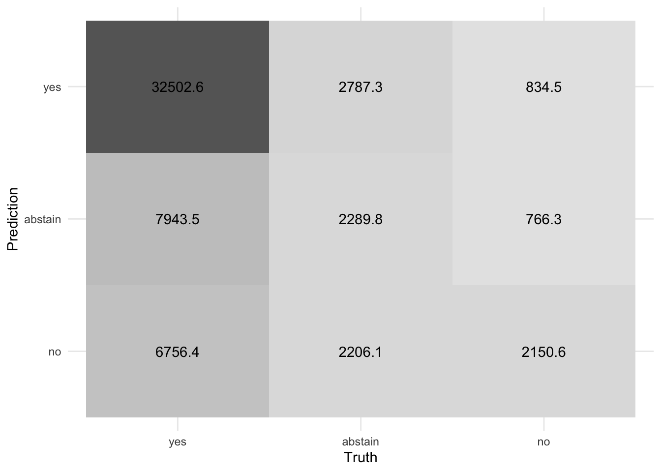
Acknowledgments
- Dataset and some modeling steps derived from Dimensionality reduction of #TidyTuesday United Nations voting patterns by Julia Silge and licensed under a Creative Commons Attribution-ShareAlike 4.0 International (CC BY-SA) License.
Session information
sessioninfo::session_info()─ Session info ───────────────────────────────────────────────────────────────
setting value
version R version 4.3.2 (2023-10-31)
os macOS Ventura 13.6.6
system aarch64, darwin20
ui X11
language (EN)
collate en_US.UTF-8
ctype en_US.UTF-8
tz America/New_York
date 2024-04-29
pandoc 3.1.1 @ /Applications/RStudio.app/Contents/Resources/app/quarto/bin/tools/ (via rmarkdown)
─ Packages ───────────────────────────────────────────────────────────────────
package * version date (UTC) lib source
backports 1.4.1 2021-12-13 [1] CRAN (R 4.3.0)
broom * 1.0.5 2023-06-09 [1] CRAN (R 4.3.0)
class 7.3-22 2023-05-03 [1] CRAN (R 4.3.2)
cli 3.6.2 2023-12-11 [1] CRAN (R 4.3.1)
codetools 0.2-19 2023-02-01 [1] CRAN (R 4.3.2)
colorspace 2.1-0 2023-01-23 [1] CRAN (R 4.3.0)
data.table 1.15.4 2024-03-30 [1] CRAN (R 4.3.1)
dials * 1.2.1 2024-02-22 [1] CRAN (R 4.3.1)
DiceDesign 1.10 2023-12-07 [1] CRAN (R 4.3.1)
digest 0.6.35 2024-03-11 [1] CRAN (R 4.3.1)
discrim * 1.0.1 2023-03-08 [1] CRAN (R 4.3.0)
dplyr * 1.1.4 2023-11-17 [1] CRAN (R 4.3.1)
ellipsis 0.3.2 2021-04-29 [1] CRAN (R 4.3.0)
embed * 1.1.4 2024-03-20 [1] CRAN (R 4.3.1)
evaluate 0.23 2023-11-01 [1] CRAN (R 4.3.1)
fansi 1.0.6 2023-12-08 [1] CRAN (R 4.3.1)
farver 2.1.1 2022-07-06 [1] CRAN (R 4.3.0)
fastmap 1.1.1 2023-02-24 [1] CRAN (R 4.3.0)
forcats * 1.0.0 2023-01-29 [1] CRAN (R 4.3.0)
foreach 1.5.2 2022-02-02 [1] CRAN (R 4.3.0)
furrr 0.3.1 2022-08-15 [1] CRAN (R 4.3.0)
future 1.33.2 2024-03-26 [1] CRAN (R 4.3.1)
future.apply 1.11.2 2024-03-28 [1] CRAN (R 4.3.1)
generics 0.1.3 2022-07-05 [1] CRAN (R 4.3.0)
ggplot2 * 3.5.1 2024-04-23 [1] CRAN (R 4.3.1)
globals 0.16.3 2024-03-08 [1] CRAN (R 4.3.1)
glue 1.7.0 2024-01-09 [1] CRAN (R 4.3.1)
gower 1.0.1 2022-12-22 [1] CRAN (R 4.3.0)
GPfit 1.0-8 2019-02-08 [1] CRAN (R 4.3.0)
gtable 0.3.5 2024-04-22 [1] CRAN (R 4.3.1)
hardhat 1.3.1 2024-02-02 [1] CRAN (R 4.3.1)
here 1.0.1 2020-12-13 [1] CRAN (R 4.3.0)
hms 1.1.3 2023-03-21 [1] CRAN (R 4.3.0)
htmltools 0.5.8.1 2024-04-04 [1] CRAN (R 4.3.1)
htmlwidgets 1.6.4 2023-12-06 [1] CRAN (R 4.3.1)
infer * 1.0.7 2024-03-25 [1] CRAN (R 4.3.1)
ipred 0.9-14 2023-03-09 [1] CRAN (R 4.3.0)
irlba 2.3.5.1 2022-10-03 [1] CRAN (R 4.3.0)
iterators 1.0.14 2022-02-05 [1] CRAN (R 4.3.0)
janeaustenr 1.0.0 2022-08-26 [1] CRAN (R 4.3.0)
jsonlite 1.8.8 2023-12-04 [1] CRAN (R 4.3.1)
knitr 1.45 2023-10-30 [1] CRAN (R 4.3.1)
labeling 0.4.3 2023-08-29 [1] CRAN (R 4.3.0)
lattice 0.21-9 2023-10-01 [1] CRAN (R 4.3.2)
lava 1.8.0 2024-03-05 [1] CRAN (R 4.3.1)
lhs 1.1.6 2022-12-17 [1] CRAN (R 4.3.0)
lifecycle 1.0.4 2023-11-07 [1] CRAN (R 4.3.1)
listenv 0.9.1 2024-01-29 [1] CRAN (R 4.3.1)
lubridate * 1.9.3 2023-09-27 [1] CRAN (R 4.3.1)
magrittr 2.0.3 2022-03-30 [1] CRAN (R 4.3.0)
MASS 7.3-60 2023-05-04 [1] CRAN (R 4.3.2)
Matrix 1.6-1.1 2023-09-18 [1] CRAN (R 4.3.2)
modeldata * 1.3.0 2024-01-21 [1] CRAN (R 4.3.1)
munsell 0.5.1 2024-04-01 [1] CRAN (R 4.3.1)
nnet 7.3-19 2023-05-03 [1] CRAN (R 4.3.2)
parallelly 1.37.1 2024-02-29 [1] CRAN (R 4.3.1)
parsnip * 1.2.1 2024-03-22 [1] CRAN (R 4.3.1)
pillar 1.9.0 2023-03-22 [1] CRAN (R 4.3.0)
pkgconfig 2.0.3 2019-09-22 [1] CRAN (R 4.3.0)
prodlim 2023.08.28 2023-08-28 [1] CRAN (R 4.3.0)
purrr * 1.0.2 2023-08-10 [1] CRAN (R 4.3.0)
R6 2.5.1 2021-08-19 [1] CRAN (R 4.3.0)
Rcpp 1.0.12 2024-01-09 [1] CRAN (R 4.3.1)
RcppAnnoy 0.0.22 2024-01-23 [1] CRAN (R 4.3.1)
readr * 2.1.5 2024-01-10 [1] CRAN (R 4.3.1)
recipes * 1.0.10 2024-02-18 [1] CRAN (R 4.3.1)
rlang 1.1.3 2024-01-10 [1] CRAN (R 4.3.1)
rmarkdown 2.26 2024-03-05 [1] CRAN (R 4.3.1)
ROSE 0.0-4 2021-06-14 [1] CRAN (R 4.3.0)
rpart * 4.1.21 2023-10-09 [1] CRAN (R 4.3.2)
rprojroot 2.0.4 2023-11-05 [1] CRAN (R 4.3.1)
rsample * 1.2.1 2024-03-25 [1] CRAN (R 4.3.1)
rstudioapi 0.16.0 2024-03-24 [1] CRAN (R 4.3.1)
scales * 1.3.0 2023-11-28 [1] CRAN (R 4.3.1)
sessioninfo 1.2.2 2021-12-06 [1] CRAN (R 4.3.0)
SnowballC 0.7.1 2023-04-25 [1] CRAN (R 4.3.0)
stringi 1.8.3 2023-12-11 [1] CRAN (R 4.3.1)
stringr * 1.5.1 2023-11-14 [1] CRAN (R 4.3.1)
survival 3.5-7 2023-08-14 [1] CRAN (R 4.3.2)
themis * 1.0.2 2023-08-14 [1] CRAN (R 4.3.0)
tibble * 3.2.1 2023-03-20 [1] CRAN (R 4.3.0)
tidymodels * 1.2.0 2024-03-25 [1] CRAN (R 4.3.1)
tidyr * 1.3.1 2024-01-24 [1] CRAN (R 4.3.1)
tidyselect 1.2.1 2024-03-11 [1] CRAN (R 4.3.1)
tidytext * 0.4.1 2023-01-07 [1] CRAN (R 4.3.0)
tidyverse * 2.0.0 2023-02-22 [1] CRAN (R 4.3.0)
timechange 0.3.0 2024-01-18 [1] CRAN (R 4.3.1)
timeDate 4032.109 2023-12-14 [1] CRAN (R 4.3.1)
tokenizers 0.3.0 2022-12-22 [1] CRAN (R 4.3.0)
tune * 1.2.1 2024-04-18 [1] CRAN (R 4.3.1)
tzdb 0.4.0 2023-05-12 [1] CRAN (R 4.3.0)
unvotes * 0.3.0 2024-04-24 [1] local
utf8 1.2.4 2023-10-22 [1] CRAN (R 4.3.1)
uwot 0.1.16 2023-06-29 [1] CRAN (R 4.3.0)
vctrs 0.6.5 2023-12-01 [1] CRAN (R 4.3.1)
viridisLite 0.4.2 2023-05-02 [1] CRAN (R 4.3.0)
withr 3.0.0 2024-01-16 [1] CRAN (R 4.3.1)
workflows * 1.1.4 2024-02-19 [1] CRAN (R 4.3.1)
workflowsets * 1.1.0 2024-03-21 [1] CRAN (R 4.3.1)
xfun 0.43 2024-03-25 [1] CRAN (R 4.3.1)
yaml 2.3.8 2023-12-11 [1] CRAN (R 4.3.1)
yardstick * 1.3.1 2024-03-21 [1] CRAN (R 4.3.1)
[1] /Library/Frameworks/R.framework/Versions/4.3-arm64/Resources/library
──────────────────────────────────────────────────────────────────────────────Footnotes
Note this is an updated version which includes General Assembly votes through early 2023.↩︎