library(tidyverse)
library(tidytext)
library(taylor)
library(tayloRswift)
library(textdata)
library(scales)

theme_set(theme_minimal())Sentiment analysis of song lyrics (Taylor’s Version)
Suggested answers
Application exercise
Answers
Taylor Swift is one of the most recognizable and popular recording artists on the planet. She is also a prolific songwriter, having written or co-written every song on each of her eleven studio albums. Currently she is smashing records on her Eras concert tour.
Taylor Swift’s music is known for its emotional depth and relatability. Her lyrics often touch on themes of love, heartbreak, and personal growth, and her music has shifted substantially over the years through different genres and styles.
In this application exercise we will use the taylor package to analyze the lyrics of Taylor Swift’s songs and attempt to answer the question: has Taylor Swift gotten angrier over time?
The package contains a data frame taylor_albums with information about each of her studio albums, including the release date, the number of tracks, and the album cover art. The package also contains a data frame taylor_album_songs with the lyrics of each song from her official studio albums.1
Import Taylor Swift lyrics
We can load the relevant data files directly from the taylor package.
Note
While we can stan artists owning their own master recordings, since our analysis is going to be on Taylor Swift’s chronological arc we need to focus purely on the original studio recordings.
library(taylor)

data("taylor_album_songs")
data("taylor_albums")

# examine original studio release albums only
taylor_album_songs_orig <- taylor_all_songs |>
  select(album_name, track_number, track_name, lyrics) |>
  # filter to full studio albums
  semi_join(y = taylor_albums |>
    filter(!ep)) |>
  # exclude rereleases
  filter(!str_detect(string = album_name, pattern = "Taylor's Version")) |>
  # order albums by release date
  mutate(album_name = factor(x = album_name, levels = taylor_albums$album_name))
taylor_album_songs_orig
# A tibble: 213 × 4
album_name track_number track_name lyrics
<fct> <int> <chr> <list>
1 Taylor Swift 1 Tim McGraw <tibble [55 × 4]>
2 Taylor Swift 2 Picture To Burn <tibble [33 × 4]>
3 Taylor Swift 3 Teardrops On My Guitar <tibble [36 × 4]>
4 Taylor Swift 4 A Place In This World <tibble [27 × 4]>
5 Taylor Swift 5 Cold As You <tibble [24 × 4]>
6 Taylor Swift 6 The Outside <tibble [37 × 4]>
7 Taylor Swift 7 Tied Together With A Smile <tibble [36 × 4]>
8 Taylor Swift 8 Stay Beautiful <tibble [51 × 4]>
9 Taylor Swift 9 Should've Said No <tibble [44 × 4]>
10 Taylor Swift 10 Mary's Song (Oh My My My) <tibble [38 × 4]>
# ℹ 203 more rowsConvert to tidytext format
Currently, taylor_album_songs is stored as one-row-song, with the lyrics nested in a list-column where each element is a tibble with one-row-per-line. The definition of a single “line” is somewhat arbitrary. For substantial analysis, we will convert the corpus to a tidy-text data frame of one-row-per-token.
Your turn: Use unnest_tokens() to tokenize the text into words (unigrams).
Note
Remember that by default, unnest_tokens() automatically converts all text to lowercase and strips out punctuation.
# tokenize taylor lyrics
taylor_lyrics <- taylor_album_songs_orig |>
  # select relevant columns
  select(album_name, track_number, track_name, lyrics) |>
  # unnest the list-column to one-row-per-song-per-line
  unnest(col = lyrics) |>
  # now tokenize the lyrics
  unnest_tokens(output = word, input = lyric)
taylor_lyrics
# A tibble: 77,460 × 7
album_name track_number track_name line element element_artist word
<fct> <int> <chr> <int> <chr> <chr> <chr>
1 Taylor Swift 1 Tim McGraw 1 Verse 1 Taylor Swift he
2 Taylor Swift 1 Tim McGraw 1 Verse 1 Taylor Swift said
3 Taylor Swift 1 Tim McGraw 1 Verse 1 Taylor Swift the
4 Taylor Swift 1 Tim McGraw 1 Verse 1 Taylor Swift way
5 Taylor Swift 1 Tim McGraw 1 Verse 1 Taylor Swift my
6 Taylor Swift 1 Tim McGraw 1 Verse 1 Taylor Swift blue
7 Taylor Swift 1 Tim McGraw 1 Verse 1 Taylor Swift eyes
8 Taylor Swift 1 Tim McGraw 1 Verse 1 Taylor Swift shined
9 Taylor Swift 1 Tim McGraw 2 Verse 1 Taylor Swift put
10 Taylor Swift 1 Tim McGraw 2 Verse 1 Taylor Swift those
# ℹ 77,450 more rowsInitial review and exploration
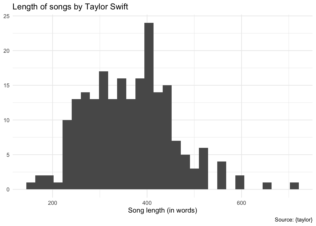
Length of songs by words
Demo: An initial check reveals the length of each song in terms of the number of words in its lyrics.
taylor_lyrics |>
  count(album_name, track_number, track_name) |>
  ggplot(mapping = aes(x = n)) +
  geom_histogram() +
  labs(
    title = "Length of songs by Taylor Swift",
    x = "Song length (in words)",
    y = NULL,
    caption = "Source: {taylor}"
  )
Stop words
Generic stop words
Of course not all words are equally important. Consider the 10 most frequent words in the lyrics:
taylor_lyrics |>
  count(word, sort = TRUE)
# A tibble: 4,505 × 2
word n
<chr> <int>
1 you 3442
2 i 3309
3 the 2757
4 and 2047
5 to 1367
6 me 1345
7 a 1315
8 it 1206
9 in 1168
10 my 1142
# ℹ 4,495 more rowsThese are not particularly informative.
Your turn: Remove stop words from the tokenized lyrics. Use the SMART stop words list.
# get a set of stop words
get_stopwords(source = "smart")
# A tibble: 571 × 2
word lexicon
<chr> <chr>
1 a smart
2 a's smart
3 able smart
4 about smart
5 above smart
6 according smart
7 accordingly smart
8 across smart
9 actually smart
10 after smart
# ℹ 561 more rows# remove stop words
taylor_tidy <- anti_join(x = taylor_lyrics, y = get_stopwords(source = "smart"))
taylor_tidy# A tibble: 25,095 × 7
album_name track_number track_name line element element_artist word
<fct> <int> <chr> <int> <chr> <chr> <chr>
1 Taylor Swift 1 Tim McGraw 1 Verse 1 Taylor Swift blue
2 Taylor Swift 1 Tim McGraw 1 Verse 1 Taylor Swift eyes
3 Taylor Swift 1 Tim McGraw 1 Verse 1 Taylor Swift shined
4 Taylor Swift 1 Tim McGraw 2 Verse 1 Taylor Swift put
5 Taylor Swift 1 Tim McGraw 2 Verse 1 Taylor Swift georgia
6 Taylor Swift 1 Tim McGraw 2 Verse 1 Taylor Swift stars
7 Taylor Swift 1 Tim McGraw 2 Verse 1 Taylor Swift shame
8 Taylor Swift 1 Tim McGraw 2 Verse 1 Taylor Swift night
9 Taylor Swift 1 Tim McGraw 3 Verse 1 Taylor Swift lie
10 Taylor Swift 1 Tim McGraw 4 Verse 1 Taylor Swift boy
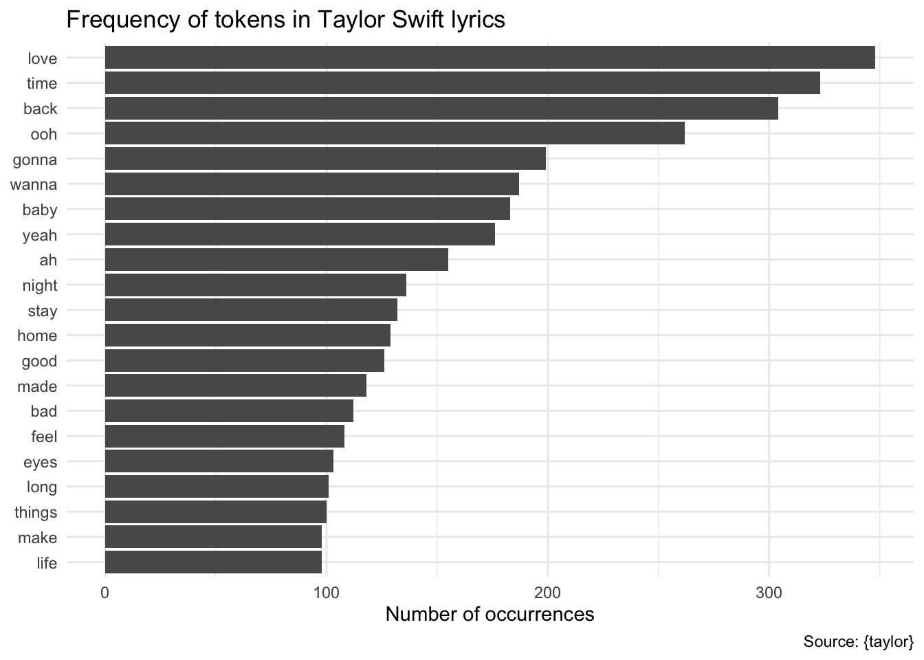
# ℹ 25,085 more rows# what are the most common words now?
taylor_tidy |>
count(word) |>
slice_max(n = 20, order_by = n) |>
mutate(word = fct_reorder(.f = word, .x = n)) |>
ggplot(aes(x = n, y = word)) +
geom_col() +
labs(
title = "Frequency of tokens in Taylor Swift lyrics",
x = "Number of occurrences",
y = NULL,
caption = "Source: {taylor}"
)
This removes 52,365 words from the corpus.
Domain-specific stop words
While this takes care of generic stop words, we can also identify domain-specific stop words. For example, Taylor Swift’s lyrics are full of interjections and exclamations that are not particularly informative. We can identify these and remove them from the corpus.
Your turn: Use the custom set of domain-specific stop words and remove them from the tokens data frame.
# domain-specific stop words
# source: https://rpubs.com/RosieB/642806
taylor_stop_words <- c(
  "oh", "ooh", "eh", "ha", "mmm", "mm", "yeah", "ah",
  "hey", "eeh", "uuh", "uh", "la", "da", "di", "ra",
  "huh", "hu", "whoa", "gonna", "wanna", "gotta", "em"
)

taylor_tidy <- taylor_lyrics |>
  anti_join(get_stopwords(source = "smart")) |>
  filter(!word %in% taylor_stop_words)
taylor_tidy
# A tibble: 23,509 × 7
album_name track_number track_name line element element_artist word
<fct> <int> <chr> <int> <chr> <chr> <chr>
1 Taylor Swift 1 Tim McGraw 1 Verse 1 Taylor Swift blue
2 Taylor Swift 1 Tim McGraw 1 Verse 1 Taylor Swift eyes
3 Taylor Swift 1 Tim McGraw 1 Verse 1 Taylor Swift shined
4 Taylor Swift 1 Tim McGraw 2 Verse 1 Taylor Swift put
5 Taylor Swift 1 Tim McGraw 2 Verse 1 Taylor Swift georgia
6 Taylor Swift 1 Tim McGraw 2 Verse 1 Taylor Swift stars
7 Taylor Swift 1 Tim McGraw 2 Verse 1 Taylor Swift shame
8 Taylor Swift 1 Tim McGraw 2 Verse 1 Taylor Swift night
9 Taylor Swift 1 Tim McGraw 3 Verse 1 Taylor Swift lie
10 Taylor Swift 1 Tim McGraw 4 Verse 1 Taylor Swift boy
# ℹ 23,499 more rowstaylor_tidy |>
count(word, sort = TRUE)# A tibble: 4,105 × 2
word n
<chr> <int>
1 love 348
2 time 323
3 back 304
4 baby 183
5 night 136
6 stay 132
7 home 129
8 good 126
9 made 118
10 bad 112
# ℹ 4,095 more rowsHow do we measure anger? Implementing dictionary-based sentiment analysis
Sentiment analysis utilizes the text of the lyrics to classify content as positive or negative. Dictionary-based methods use pre-generated lexicons of words independently coded as positive/negative. We can combine one of these dictionaries with the Taylor Swift tidy-text data frame using inner_join() to identify words with sentimental affect, and further analyze trends.
Your turn: Use the afinn dictionary which classifies 2,477 words on a scale of \([-5, +5]\). Join the sentiment dictionary with the tokenized lyrics and only retain words that are defined in the dictionary.
# afinn dictionary
get_sentiments(lexicon = "afinn")
# A tibble: 2,477 × 2
word value
<chr> <dbl>
1 abandon -2
2 abandoned -2
3 abandons -2
4 abducted -2
5 abduction -2
6 abductions -2
7 abhor -3
8 abhorred -3
9 abhorrent -3
10 abhors -3
# ℹ 2,467 more rows# how many words for each value?
get_sentiments(lexicon = "afinn") |>
count(value)# A tibble: 11 × 2
value n
<dbl> <int>
1 -5 16
2 -4 43
3 -3 264
4 -2 966
5 -1 309
6 0 1
7 1 208
8 2 448
9 3 172
10 4 45
11 5 5# join with sentiment dictionary, drop words which are not defined
taylor_afinn <- taylor_tidy |>
inner_join(y = get_sentiments(lexicon = "afinn"))
taylor_afinn# A tibble: 4,553 × 8
album_name track_number track_name line element element_artist word value
<fct> <int> <chr> <int> <chr> <chr> <chr> <dbl>
1 Taylor Swift 1 Tim McGraw 2 Verse 1 Taylor Swift shame -2
2 Taylor Swift 1 Tim McGraw 5 Verse 1 Taylor Swift stuck -2
3 Taylor Swift 1 Tim McGraw 10 Chorus Taylor Swift hope 2
4 Taylor Swift 1 Tim McGraw 10 Chorus Taylor Swift favo… 2
5 Taylor Swift 1 Tim McGraw 13 Chorus Taylor Swift happ… 3
6 Taylor Swift 1 Tim McGraw 14 Chorus Taylor Swift hope 2
7 Taylor Swift 1 Tim McGraw 18 Chorus Taylor Swift hope 2
8 Taylor Swift 1 Tim McGraw 19 Verse 2 Taylor Swift tears -2
9 Taylor Swift 1 Tim McGraw 20 Verse 2 Taylor Swift god 1
10 Taylor Swift 1 Tim McGraw 25 Verse 2 Taylor Swift hard -1
# ℹ 4,543 more rowsSentimental affect of each song
Your turn: Examine the sentiment of each song individually by calculating the average sentiment of each word in the song. What are the top-5 most positive and negative songs?
taylor_afinn_sum <- taylor_afinn |>
  summarize(sent = mean(value), .by = c(album_name, track_name))

slice_max(.data = taylor_afinn_sum, n = 5, order_by = sent)
# A tibble: 7 × 3
album_name track_name sent
<fct> <chr> <dbl>
1 Taylor Swift A Perfectly Good Heart 2.89
2 Taylor Swift Stay Beautiful 2.36
3 1989 You Are In Love 2.12
4 THE TORTURED POETS DEPARTMENT I Can Fix Him (No Really I Can) 2.09
5 reputation This Is Why We Can't Have Nice Things 2
6 Lover London Boy 2
7 Lover It's Nice To Have A Friend 2 slice_min(.data = taylor_afinn_sum, n = 5, order_by = sent)# A tibble: 5 × 3
album_name track_name sent
<fct> <chr> <dbl>
1 THE TORTURED POETS DEPARTMENT Cassandra -2.62
2 THE TORTURED POETS DEPARTMENT Down Bad -2.60
3 1989 Shake It Off -2.56
4 Midnights Lavender Haze -2.38
5 1989 How You Get The Girl -2.17Shake It Off
However, this also illustrates some problems with dictionary-based sentiment analysis. Consider “Shake It Off (Taylor’s Version)” which is scored as a NaN.
Your turn: What are the most positive and negative words in “Shake It Off”? Do these seem reflective of the song’s overall sentiment?
# what's up with shake it off?
taylor_afinn |>
  filter(track_name == "Shake It Off") |>
  count(word, value) |>
  arrange(-value)
# A tibble: 11 × 3
word value n
<chr> <dbl> <int>
1 good 3 1
2 god 1 1
3 stop -1 4
4 dirty -2 2
5 miss -2 1
6 sick -2 1
7 cheats -3 1
8 fake -3 18
9 hate -3 16
10 haters -3 4
11 liars -3 1Add response here. Would most listeners classify this song as full of negativity? Probs not. Herein lies the problem with dictionary-based methods. The AFINN lexicon codes “fake” and “hate” as negative terms, even though in this context they are being used more positively – the singer is shaking off the haters and going her own way in life.
This is a common problem with dictionary-based methods, and why it is important to carefully consider the context of the text being analyzed.
Sentimental affect of each album
Your turn: Calculate the average sentimental affect for each album, and examine the general disposition of each album based on their overall positive/negative affect. Report on any trends you observe.
# errorbar plot
taylor_afinn |>
  # calculate average sentiment by album with standard error
  summarize(
    sent = mean(value),
    se = sd(value) / sqrt(n()),
    .by = album_name
  ) |>
  # reverse album order for vertical plot
  mutate(album_name = fct_rev(f = album_name)) |>
  # generate plot
  ggplot(mapping = aes(y = album_name, x = sent)) +
  geom_pointrange(mapping = aes(
    xmin = sent - 2 * se,
    xmax = sent + 2 * se
  )) +
  labs(
    title = "Emotional affect in Taylor Swift albums",
    x = "Average sentiment",
    y = NULL,
    caption = "Source: {taylor}"
  )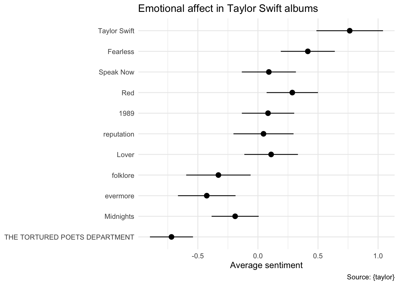
Add response here. A trend is beginning to emerge - Taylor Swift’s earlier albums are more positive, while her later albums are more negative. This is consistent with the narrative that Taylor Swift’s music has become more mature and introspective over time, but “anger” is not the same as “negativity”.
Varying types of sentiment
Your turn: tidytext and textdata include multiple sentiment dictionaries for different types of sentiment. Use the NRC Affect Intensity Lexicon to score each of Taylor Swift’s songs based on four basic emotions (anger, fear, sadness, and joy), then calculate the sum total for each type of affect by album, standardized by the number of affective words in each album.
Tip
Use lexicon_nrc_eil() from textdata to download the sentiment dictionary.
# NRC emotion intensity lexicon
lexicon_nrc_eil()
# A tibble: 5,814 × 3
term score AffectDimension
<chr> <dbl> <chr>
1 outraged 0.964 anger
2 brutality 0.959 anger
3 hatred 0.953 anger
4 hateful 0.94 anger
5 terrorize 0.939 anger
6 infuriated 0.938 anger
7 violently 0.938 anger
8 furious 0.929 anger
9 enraged 0.927 anger
10 furiously 0.927 anger
# ℹ 5,804 more rowstaylor_tidy |>
# join with sentiment dictionary
inner_join(
y = lexicon_nrc_eil(), by = join_by(word == term),
relationship = "many-to-many"
) |>
# calculate cumulative affect for each album and dimension
summarize(
score = sum(score),
n = n(),
.by = c(album_name, AffectDimension)
) |>
# determine the total number of affective terms per album and standardize
mutate(n = sum(n), .by = album_name) |>
mutate(
score_norm = score / n,
album_name = fct_rev(album_name)
) |>
# visualize using a bar plot
ggplot(mapping = aes(x = score_norm, y = album_name)) +
geom_col() +
facet_wrap(
facets = vars(AffectDimension)
) +
labs(
title = "Sentimental affect (by type) in Taylor Swift albums",
subtitle = "Original studio albums",
x = "Affect intensity (normalized per token)",
y = NULL,
caption = "Source: {taylor}"
)
Add response here. Relative levels of anger, fear, and sadness have remained roughly the same across albums, whereas joy has decreased over time. This is consistent with the narrative that Taylor Swift’s music has become more introspective and less joyful over time.
Fuck it, let’s build a dictionary ourselves
What if we operationalize “anger” purely on the frequency of cursing in Taylor Swift’s songs? We can generate our own custom curse word dictionary2 and examine the relative usage of these words across Taylor Swift’s albums.
Your turn: Use the curse word dictionary to calculate how often Taylor Swift curses across her studio albums. Identify any relevant trends.
# curse word dictionary
taylor_curses <- c(
  "whore", "damn", "goddamn", "hell",
  "bitch", "shit", "fuck", "dickhead"
)

taylor_tidy |>
  # only keep words that appear in curse word dictionary
  filter(word %in% taylor_curses) |>
  # format columns for plotting
  mutate(
    word = fct_infreq(f = word),
    album_name = str_wrap(album_name, 20) |>
      fct_inorder() |>
      fct_rev()
  ) |>
  # horizontal bar chart
  ggplot(mapping = aes(y = album_name, fill = word)) +
  geom_bar(color = "white") +
  # use a Taylor Swift color palette
  scale_fill_taylor_d(album = "1989", guide = guide_legend(nrow = 1, rev = TRUE)) +
  labs(
    title = "Swear words in Taylor Swift albums",
    x = "Frequency count",
    y = NULL,
    fill = NULL,
    caption = "Source: {taylor}"
  ) +
  # format legend to not get cut off on the side
  theme(
    legend.position = "top",
    legend.text.position = "bottom"
  )
Add response here. Her last four albums have seen a dramatic increase in the usage of curse words. “Damn”/“goddamn”, “shit”, and “fuck” seem to account for the vast majority of the usage.
Session information
sessioninfo::session_info()─ Session info ───────────────────────────────────────────────────────────────
setting value
version R version 4.3.2 (2023-10-31)
os macOS Ventura 13.6.6
system aarch64, darwin20
ui X11
language (EN)
collate en_US.UTF-8
ctype en_US.UTF-8
tz America/New_York
date 2024-05-02
pandoc 3.1.11 @ /Applications/RStudio.app/Contents/Resources/app/quarto/bin/tools/aarch64/ (via rmarkdown)
─ Packages ───────────────────────────────────────────────────────────────────
package * version date (UTC) lib source
cli 3.6.2 2023-12-11 [1] CRAN (R 4.3.1)
colorspace 2.1-0 2023-01-23 [1] CRAN (R 4.3.0)
digest 0.6.35 2024-03-11 [1] CRAN (R 4.3.1)
dplyr * 1.1.4 2023-11-17 [1] CRAN (R 4.3.1)
evaluate 0.23 2023-11-01 [1] CRAN (R 4.3.1)
fansi 1.0.6 2023-12-08 [1] CRAN (R 4.3.1)
farver 2.1.1 2022-07-06 [1] CRAN (R 4.3.0)
fastmap 1.1.1 2023-02-24 [1] CRAN (R 4.3.0)
forcats * 1.0.0 2023-01-29 [1] CRAN (R 4.3.0)
fs 1.6.3 2023-07-20 [1] CRAN (R 4.3.0)
generics 0.1.3 2022-07-05 [1] CRAN (R 4.3.0)
ggplot2 * 3.5.1 2024-04-23 [1] CRAN (R 4.3.1)
glue 1.7.0 2024-01-09 [1] CRAN (R 4.3.1)
gtable 0.3.5 2024-04-22 [1] CRAN (R 4.3.1)
here 1.0.1 2020-12-13 [1] CRAN (R 4.3.0)
hms 1.1.3 2023-03-21 [1] CRAN (R 4.3.0)
htmltools 0.5.8.1 2024-04-04 [1] CRAN (R 4.3.1)
htmlwidgets 1.6.4 2023-12-06 [1] CRAN (R 4.3.1)
janeaustenr 1.0.0 2022-08-26 [1] CRAN (R 4.3.0)
jsonlite 1.8.8 2023-12-04 [1] CRAN (R 4.3.1)
knitr 1.45 2023-10-30 [1] CRAN (R 4.3.1)
labeling 0.4.3 2023-08-29 [1] CRAN (R 4.3.0)
lattice 0.21-9 2023-10-01 [1] CRAN (R 4.3.2)
lifecycle 1.0.4 2023-11-07 [1] CRAN (R 4.3.1)
lubridate * 1.9.3 2023-09-27 [1] CRAN (R 4.3.1)
magrittr 2.0.3 2022-03-30 [1] CRAN (R 4.3.0)
Matrix 1.6-1.1 2023-09-18 [1] CRAN (R 4.3.2)
munsell 0.5.1 2024-04-01 [1] CRAN (R 4.3.1)
pillar 1.9.0 2023-03-22 [1] CRAN (R 4.3.0)
pkgconfig 2.0.3 2019-09-22 [1] CRAN (R 4.3.0)
purrr * 1.0.2 2023-08-10 [1] CRAN (R 4.3.0)
R6 2.5.1 2021-08-19 [1] CRAN (R 4.3.0)
rappdirs 0.3.3 2021-01-31 [1] CRAN (R 4.3.0)
Rcpp 1.0.12 2024-01-09 [1] CRAN (R 4.3.1)
readr * 2.1.5 2024-01-10 [1] CRAN (R 4.3.1)
rlang 1.1.3 2024-01-10 [1] CRAN (R 4.3.1)
rmarkdown 2.26 2024-03-05 [1] CRAN (R 4.3.1)
rprojroot 2.0.4 2023-11-05 [1] CRAN (R 4.3.1)
rstudioapi 0.16.0 2024-03-24 [1] CRAN (R 4.3.1)
scales * 1.3.0 2023-11-28 [1] CRAN (R 4.3.1)
sessioninfo 1.2.2 2021-12-06 [1] CRAN (R 4.3.0)
SnowballC 0.7.1 2023-04-25 [1] CRAN (R 4.3.0)
stopwords 2.3 2021-10-28 [1] CRAN (R 4.3.0)
stringi 1.8.3 2023-12-11 [1] CRAN (R 4.3.1)
stringr * 1.5.1 2023-11-14 [1] CRAN (R 4.3.1)
taylor * 3.0.0.9000 2024-04-19 [1] Github (wjakethompson/taylor@9b3181e)
tayloRswift * 0.2.0 2023-11-02 [1] Github (asteves/tayloRswift@445a16a)
textdata * 0.4.4 2022-09-02 [1] CRAN (R 4.3.0)
tibble * 3.2.1 2023-03-20 [1] CRAN (R 4.3.0)
tidyr * 1.3.1 2024-01-24 [1] CRAN (R 4.3.1)
tidyselect 1.2.1 2024-03-11 [1] CRAN (R 4.3.1)
tidytext * 0.4.1 2023-01-07 [1] CRAN (R 4.3.0)
tidyverse * 2.0.0 2023-02-22 [1] CRAN (R 4.3.0)
timechange 0.3.0 2024-01-18 [1] CRAN (R 4.3.1)
tokenizers 0.3.0 2022-12-22 [1] CRAN (R 4.3.0)
tzdb 0.4.0 2023-05-12 [1] CRAN (R 4.3.0)
utf8 1.2.4 2023-10-22 [1] CRAN (R 4.3.1)
vctrs 0.6.5 2023-12-01 [1] CRAN (R 4.3.1)
withr 3.0.0 2024-01-16 [1] CRAN (R 4.3.1)
xfun 0.43 2024-03-25 [1] CRAN (R 4.3.1)
yaml 2.3.8 2023-12-11 [1] CRAN (R 4.3.1)
[1] /Library/Frameworks/R.framework/Versions/4.3-arm64/Resources/library
──────────────────────────────────────────────────────────────────────────────Footnotes
This excludes singles released separately from an album as well as non-Taylor-owned albums that have a Taylor-owned alternative (e.g., Fearless is excluded in favor of Fearless (Taylor’s Version)).↩︎
Courtesy of stephsmithio on r/dataisbeautiful↩︎