library(tidyverse)
library(wordcloud)
library(tidytext)
library(scales)
library(viridis)

# set default seed and theme
set.seed(123)
theme_set(theme_minimal())Securely storing API keys
Tutorial
Application programming interface
What are API keys and how to store them securely for R packages.
What are API keys?
An application programming interface (API) key is a unique identifier used to authenticate and authorize a user, developer, or calling program to an API.1 API keys are used to track and control how the API is being used, for example to prevent malicious use or abuse of the API. The API key often acts as both a unique identifier and a secret token for authentication, and is assigned a set of access that is specific to the identity that is associated with it.
Depending on how the API is set up, you may need to include your API key in every request you make, or you may only need to include it once to get a token that you can use for subsequent requests. In either case, you should never share your API key with anyone else. If you do, they will be able to use the API as if they were you, and you may be held responsible for any misuse of the API.
Searching geographic info: geonames
library(geonames)API authentication
There are a few things we need to do to be able to use this package to access the geonames API:
- Go to the geonames site and register an account.
- Click here to enable the free web service
- Tell R your geonames username. You could run the line
options(geonamesUsername = "<YOUR USER NAME>")in R. However this is insecure. We don’t want to risk committing this line and pushing it to our public GitHub page! Instead, you should create a file in the same place as your .Rproj file. To do that, run the following command from the R console:
usethis::edit_r_profile(scope = "project")This will create a special file called .Rprofile in the same directory as your .Rproj file (assuming you are working in an R project). The file should open automatically in your RStudio script editor. Add
options(geonamesUsername = "<YOUR USER NAME>")to that file, replacing <YOUR USER NAME> with your Geonames username.
Important
- Make sure your
.Rprofileends with a blank line - Make sure
.Rprofileis included in your.gitignorefile, otherwise it will be synced with Github - Restart RStudio after modifying
.Rprofilein order to load any new keys into memory - Spelling is important when you set the option in your
.Rprofile - You can do a similar process for an arbitrary package or key. For example:
# in .Rprofile
options(this_is_my_key = "XXXX")

# later, in the R script:
key <- getOption("this_is_my_key")
This is a simple means to keep your keys private, especially if you are sharing the same authentication across several projects. Remember that using .Rprofile makes your code un-reproducible. In this case, that is exactly what we want!
Using Geonames
What can we do? Get access to lots of geographical information via the various “web services”
countryInfo <- GNcountryInfo()countryInfo |>
as_tibble() |>
glimpse()Rows: 250
Columns: 18
$ continent <chr> "EU", "AS", "AS", "NA", "NA", "EU", "AS", "AF", "AN",…
$ capital <chr> "Andorra la Vella", "Abu Dhabi", "Kabul", "Saint John…
$ languages <chr> "ca", "ar-AE,fa,en,hi,ur", "fa-AF,ps,uz-AF,tk", "en-A…
$ geonameId <chr> "3041565", "290557", "1149361", "3576396", "3573511",…
$ south <chr> "42.4287475", "22.6315119400001", "29.3770645357176",…
$ isoAlpha3 <chr> "AND", "ARE", "AFG", "ATG", "AIA", "ALB", "ARM", "AGO…
$ north <chr> "42.6558875", "26.0693916590001", "38.4907920755748",…
$ fipsCode <chr> "AN", "AE", "AF", "AC", "AV", "AL", "AM", "AO", "AY",…
$ population <chr> "77006", "9630959", "37172386", "96286", "13254", "28…
$ east <chr> "1.7866939", "56.381222289", "74.8894511481168", "-61…
$ isoNumeric <chr> "020", "784", "004", "028", "660", "008", "051", "024…
$ areaInSqKm <chr> "468.0", "82880.0", "647500.0", "443.0", "102.0", "28…
$ countryCode <chr> "AD", "AE", "AF", "AG", "AI", "AL", "AM", "AO", "AQ",…
$ west <chr> "1.4135734", "51.5904085340001", "60.4720833972263", …
$ countryName <chr> "Principality of Andorra", "United Arab Emirates", "I…
$ postalCodeFormat <chr> "AD###", "", "", "", "", "####", "######", "", "", "@…
$ continentName <chr> "Europe", "Asia", "Asia", "North America", "North Ame…
$ currencyCode <chr> "EUR", "AED", "AFN", "XCD", "XCD", "ALL", "AMD", "AOA…This country info dataset is very helpful for accessing the rest of the data, because it gives us the standardized codes for country and language.
The Manifesto Project: manifestoR
The Manifesto Project collects and organizes political party manifestos from around the world. It currently covers over 1000 parties from 1945 until today in over 50 countries on five continents. We can use the manifestoR package to access the API and download those manifestos for analysis in R.
Load library and set API key
Accessing data from the Manifesto Project API requires an authentication key. You can create an account and key here. Here I store my key in .Rprofile and retrieve it using mp_setapikey().
library(manifestoR)

# retrieve API key stored in .Rprofile
mp_setapikey(key = getOption("manifesto_key"))
Once you have done this step, your API key is automatically included in every request you make to the Manifesto Project API.
Retrieve the database
mpds <- mp_maindataset()Connecting to Manifesto Project DB API...
Connecting to Manifesto Project DB API... corpus version: 2023-1 mpds# A tibble: 5,089 × 175
country countryname oecdmember eumember edate date party partyname
<dbl> <chr> <dbl> <dbl> <date> <dbl> <dbl> <chr>
1 11 Sweden 0 0 1944-09-17 194409 11220 Communist Pa…
2 11 Sweden 0 0 1944-09-17 194409 11320 Social Democ…
3 11 Sweden 0 0 1944-09-17 194409 11420 People’s Par…
4 11 Sweden 0 0 1944-09-17 194409 11620 Right Party
5 11 Sweden 0 0 1944-09-17 194409 11810 Agrarian Par…
6 11 Sweden 0 0 1948-09-19 194809 11220 Communist Pa…
7 11 Sweden 0 0 1948-09-19 194809 11320 Social Democ…
8 11 Sweden 0 0 1948-09-19 194809 11420 People’s Par…
9 11 Sweden 0 0 1948-09-19 194809 11620 Right Party
10 11 Sweden 0 0 1948-09-19 194809 11810 Agrarian Par…
# ℹ 5,079 more rows
# ℹ 167 more variables: partyabbrev <chr>, parfam <dbl>, candidatename <chr>,
# coderid <dbl>, manual <dbl>, coderyear <dbl>, testresult <dbl>,
# testeditsim <dbl>, pervote <dbl>, voteest <dbl>, presvote <dbl>,
# absseat <dbl>, totseats <dbl>, progtype <dbl>, datasetorigin <dbl>,
# corpusversion <chr>, total <dbl>, peruncod <dbl>, per101 <dbl>,
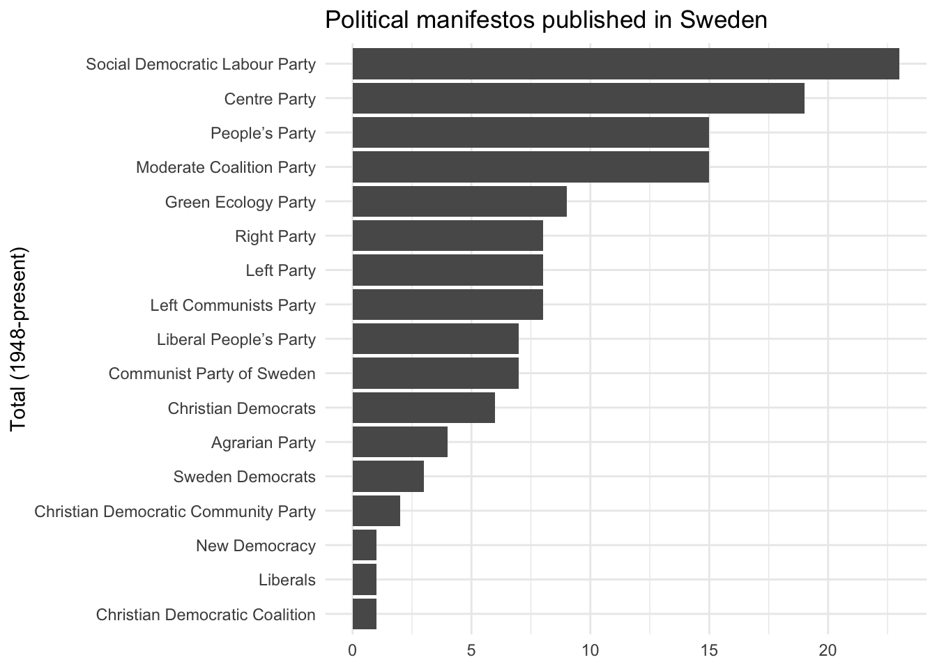
# per102 <dbl>, per103 <dbl>, per104 <dbl>, per105 <dbl>, per106 <dbl>, …mp_maindataset() includes a data frame describing each manifesto included in the database. You can use this database for some exploratory data analysis. For instance, how many manifestos have been published by each political party in Sweden?
mpds |>
  filter(countryname == "Sweden") |>
  count(partyname) |>
  mutate(partyname = fct_reorder(.f = partyname, .x = n)) |>
  ggplot(mapping = aes(x = n, y = partyname)) +
  geom_col() +
  labs(
    title = "Political manifestos published in Sweden",
    x = NULL,
    y = "Total (1948-present)"
  )
Or we can use scaling functions to identify each party manifesto on an ideological dimension. For example, how have the Democratic and Republican Party manifestos in the United States changed over time?
mpds_usa <- mpds |>
  filter(party == 61320 | party == 61620)

mpds_usa |>
  mutate(ideo = mp_scale(mpds_usa)) |>
  select(partyname, edate, ideo) |>
  ggplot(aes(edate, ideo, color = partyname)) +
  geom_line() +
  scale_color_manual(values = c("blue", "red")) +
  labs(
    title = "Ideological scaling of major US political parties",
    x = "Year",
    y = "Ideological position",
    color = NULL
  ) +
  theme(legend.position = "bottom")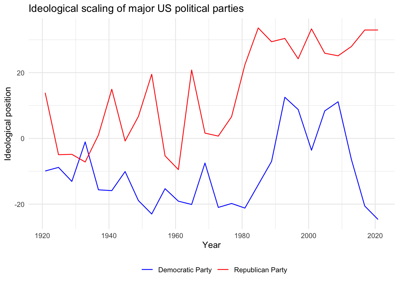
Download manifestos
mp_corpus() can be used to download the original manifestos as full text documents stored as a corpus. Once you obtain the corpus, you can perform text analysis. As an example, let’s compare the most common words in the Democratic and Republican Party manifestos from the 2020 U.S. presidential election:
# download documents
docs <- mp_corpus(countryname == "United States" & edate > as.Date("2020-01-01"))
Connecting to Manifesto Project DB API...
Connecting to Manifesto Project DB API... corpus version: 2023-1
Connecting to Manifesto Project DB API... corpus version: 2023-1
Connecting to Manifesto Project DB API... corpus version: 2023-1 docs<<ManifestoCorpus>>
Metadata: corpus specific: 0, document level (indexed): 0
Content: documents: 2# generate wordcloud of most common terms
docs |>
tidy() |>
mutate(party = factor(x = party,
levels = c(61320, 61620),
labels = c("Democratic Party", "Republican Party")
)) |>
unnest_tokens(word, text) |>
anti_join(stop_words) |>
count(party, word, sort = TRUE) |>
drop_na() |>
reshape2::acast(word ~ party, value.var = "n", fill = 0) |>
comparison.cloud(max.words = 200)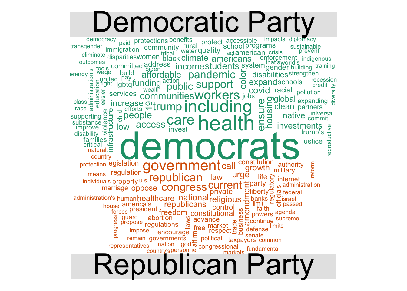
Census data with tidycensus
tidycensus provides an interface with the US Census Bureau’s decennial census and American Community APIs and returns tidy data frames with optional simple feature geometry. These APIs require a free key you can obtain here.
Rather than storing your key in .Rprofile, tidycensus includes census_api_key() which automatically stores your key in .Renviron, which is a location to store environment variables. Anything stored in .Renviron is automatically loaded anytime you initiate R on your computer, regardless of the project or file location. Once you get your key, load it:
library(tidycensus)census_api_key("YOUR API KEY GOES HERE", install = TRUE)
Tip
All future requests to the Census API using tidycensus on your computer will automatically include your key. You will not need to run census_api_key() again.
Obtaining decennial census data
get_decennial() allows you to obtain data from the 1990, 2000, 2010, and 2020 decennial US censuses. Let’s look at the number of individuals of Asian ethnicity by state in 2020:2
asia20 <- get_decennial(geography = "state", variables = "P1_006N", year = 2020)Getting data from the 2020 decennial CensusUsing the PL 94-171 Redistricting Data Summary FileNote: 2020 decennial Census data use differential privacy, a technique that
introduces errors into data to preserve respondent confidentiality.
ℹ Small counts should be interpreted with caution.
ℹ See https://www.census.gov/library/fact-sheets/2021/protecting-the-confidentiality-of-the-2020-census-redistricting-data.html for additional guidance.
This message is displayed once per session.asia20# A tibble: 52 × 4
GEOID NAME variable value
<chr> <chr> <chr> <dbl>
1 42 Pennsylvania P1_006N 510501
2 06 California P1_006N 6085947
3 54 West Virginia P1_006N 15109
4 49 Utah P1_006N 80438
5 36 New York P1_006N 1933127
6 11 District of Columbia P1_006N 33545
7 02 Alaska P1_006N 44032
8 12 Florida P1_006N 643682
9 45 South Carolina P1_006N 90466
10 38 North Dakota P1_006N 13213
# ℹ 42 more rowsThe result of get_decennial() is a tidy data frame with one row per geographic unit-variable.
GEOID- identifier for the geographical unit associated with the rowNAME- descriptive name of the geographical unitvariable- the Census variable encoded in the rowvalue- the value of the variable for that geographic unit
We can quickly visualize this data frame using ggplot2:
asia20 |>
  mutate(NAME = fct_reorder(.f = NAME, .x = value)) |>
  ggplot(mapping = aes(x = value, y = NAME)) +
  geom_point() +
  scale_x_continuous(labels = label_comma(scale_cut = cut_short_scale())) +
  labs(
    x = NULL,
    y = "Number of residents of Asian ethnicity"
  )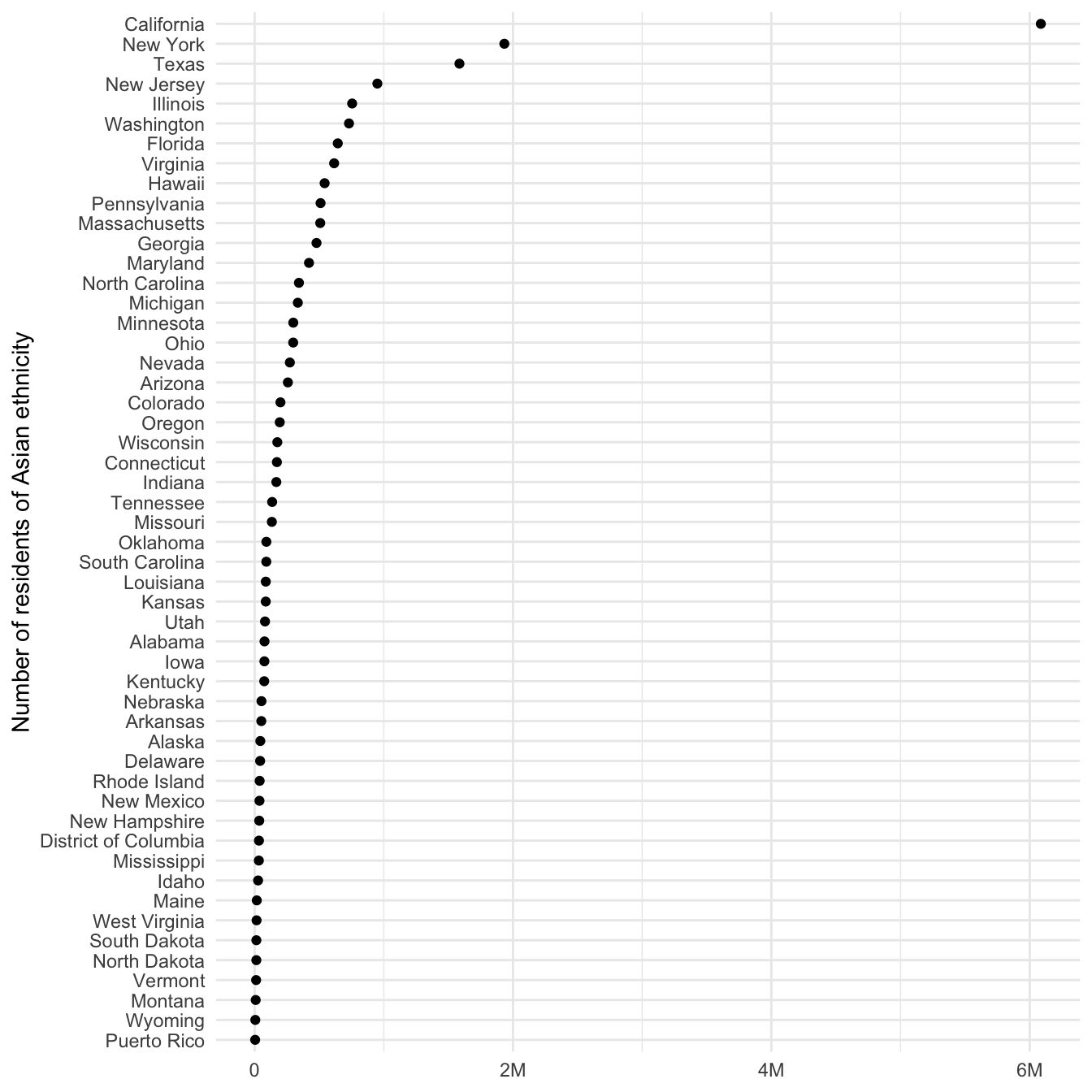
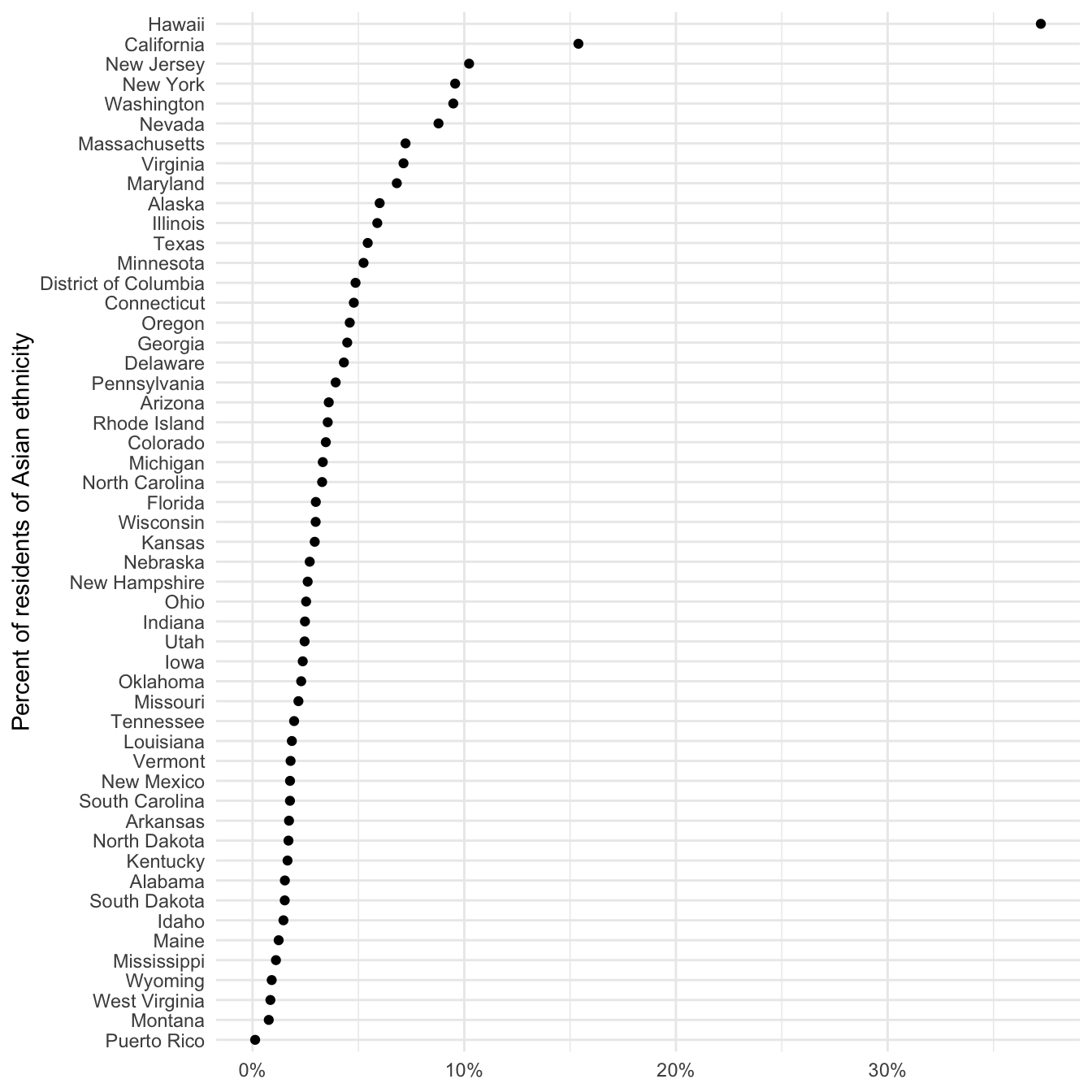
Of course this graph is not entirely useful since it is based on the raw frequency of Asian individuals. California is at the top of the list, but it is also the most populous state. Instead, we could normalize this value as a percentage of the entire state population. To do that, we need to retrieve another variable:
asia_pop <- get_decennial(
  geography = "state",
  variables = c(asian = "P1_006N", total = "P1_001N"),
  year = 2020,
  output = "wide"
)
Getting data from the 2020 decennial CensusUsing the PL 94-171 Redistricting Data Summary Fileasia_pop# A tibble: 52 × 4
GEOID NAME asian total
<chr> <chr> <dbl> <dbl>
1 42 Pennsylvania 510501 13002700
2 06 California 6085947 39538223
3 54 West Virginia 15109 1793716
4 49 Utah 80438 3271616
5 36 New York 1933127 20201249
6 11 District of Columbia 33545 689545
7 02 Alaska 44032 733391
8 12 Florida 643682 21538187
9 45 South Carolina 90466 5118425
10 38 North Dakota 13213 779094
# ℹ 42 more rowsasia_pop |>
mutate(asian_pct = asian / total,
NAME = fct_reorder(.f = NAME, .x = asian_pct)) |>
ggplot(mapping = aes(x = asian_pct, y = NAME)) +
geom_point() +
scale_x_continuous(labels = label_percent()) +
labs(
x = NULL,
y = "Percent of residents of Asian ethnicity"
)
Obtaining American Community Survey data
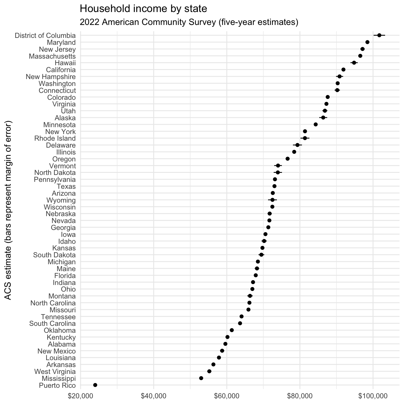
get_acs() retrieves data from the American Community Survey. This survey is administered to a sample of 3 million households on an annual basis, so the data points are estimates characterized by a margin of error. tidycensus returns both the original estimate and margin of error. Let’s get median household income data from the 2018-2012 ACS for each state.
usa_inc <- get_acs(
  geography = "state",
  variables = c(medincome = "B19013_001"),
  year = 2022
)
Getting data from the 2018-2022 5-year ACSusa_inc# A tibble: 52 × 5
GEOID NAME variable estimate moe
<chr> <chr> <chr> <dbl> <dbl>
1 01 Alabama medincome 59609 377
2 02 Alaska medincome 86370 1083
3 04 Arizona medincome 72581 450
4 05 Arkansas medincome 56335 422
5 06 California medincome 91905 277
6 08 Colorado medincome 87598 508
7 09 Connecticut medincome 90213 730
8 10 Delaware medincome 79325 1227
9 11 District of Columbia medincome 101722 1569
10 12 Florida medincome 67917 259
# ℹ 42 more rowsNow we return both an estimate column for the ACS estimate and moe for the margin of error (defaults to 90% confidence interval).
usa_inc |>
  mutate(NAME = fct_reorder(.f = NAME, .x = estimate)) |>
  ggplot(mapping = aes(x = estimate, y = NAME)) +
  geom_pointrange(mapping = aes(
    xmin = estimate - moe,
    xmax = estimate + moe
  ),
  size = .25
  ) +
  scale_x_continuous(labels = label_dollar()) +
  labs(
    title = "Household income by state",
    subtitle = "2022 American Community Survey (five-year estimates)",
    x = NULL,
    y = "ACS estimate (bars represent margin of error)"
  )
Search for variables
get_acs() or get_decennial() requires knowing the variable ID, of which there are thousands. load_variables() downloads a list of variable IDs and labels for a given Census or ACS and dataset. You can then use view() to interactively browse through and filter for variables in RStudio.
Drawing maps
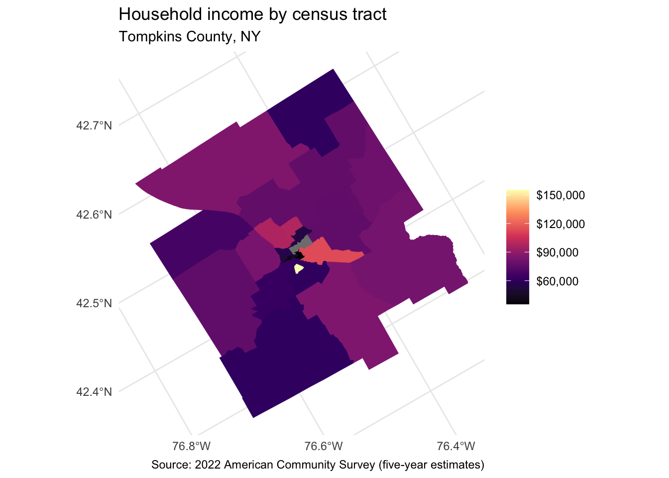
tidycensus also can return simple feature geometry for geographic units along with variables from the decennial Census or ACS, which can then be visualized using geom_sf(). Let’s look at median household income by Census tracts from the 2018-2022 ACS in Tompkins County, NY:
tompkins <- get_acs(
  state = "NY",
  county = "Tompkins",
  geography = "tract",
  variables = c(medincome = "B19013_001"),
  year = 2022,
  geometry = TRUE
)tompkinsSimple feature collection with 26 features and 5 fields
Geometry type: MULTIPOLYGON
Dimension: XY
Bounding box: xmin: -76.69666 ymin: 42.26298 xmax: -76.23782 ymax: 42.62742
Geodetic CRS: NAD83
First 10 features:
GEOID NAME variable estimate
1 36109000300 Census Tract 3; Tompkins County; New York medincome NA
2 36109000800 Census Tract 8; Tompkins County; New York medincome 52188
3 36109000100 Census Tract 1; Tompkins County; New York medincome 39512
4 36109000600 Census Tract 6; Tompkins County; New York medincome 97500
5 36109000201 Census Tract 2.01; Tompkins County; New York medincome NA
6 36109000900 Census Tract 9; Tompkins County; New York medincome 83510
7 36109000400 Census Tract 4; Tompkins County; New York medincome 53750
8 36109002300 Census Tract 23; Tompkins County; New York medincome 85295
9 36109000700 Census Tract 7; Tompkins County; New York medincome 56578
10 36109001500 Census Tract 15; Tompkins County; New York medincome 76841
moe geometry
1 NA MULTIPOLYGON (((-76.48981 4...
2 24145 MULTIPOLYGON (((-76.51474 4...
3 5060 MULTIPOLYGON (((-76.50839 4...
4 44884 MULTIPOLYGON (((-76.52701 4...
5 NA MULTIPOLYGON (((-76.48959 4...
6 11361 MULTIPOLYGON (((-76.57343 4...
7 27113 MULTIPOLYGON (((-76.48973 4...
8 16628 MULTIPOLYGON (((-76.66654 4...
9 10038 MULTIPOLYGON (((-76.51177 4...
10 20642 MULTIPOLYGON (((-76.53789 4...This looks similar to the previous output but because we set geometry = TRUE it is now a simple features data frame with a geometry column defining the geographic feature. We can visualize it using geom_sf() and viridis::scale_*_viridis() to adjust the color palette.
ggplot(data = tompkins) +
  geom_sf(mapping = aes(fill = estimate, color = estimate)) +
  coord_sf(crs = 26911) +
  scale_fill_viridis_c(
    option = "magma",
    labels = label_dollar(),
    aesthetics = c("fill", "color")
  ) +
  labs(
    title = "Household income by census tract",
    subtitle = "Tompkins County, NY",
    caption = "Source: 2022 American Community Survey (five-year estimates)",
    fill = NULL,
    color = NULL
  )
Acknowledgments
- This page is derived in part from “UBC STAT 545A and 547M”, licensed under the CC BY-NC 3.0 Creative Commons License.
Session information
sessioninfo::session_info()─ Session info ───────────────────────────────────────────────────────────────
setting value
version R version 4.3.2 (2023-10-31)
os macOS Ventura 13.5.2
system aarch64, darwin20
ui X11
language (EN)
collate en_US.UTF-8
ctype en_US.UTF-8
tz America/New_York
date 2024-03-11
pandoc 3.1.1 @ /Applications/RStudio.app/Contents/Resources/app/quarto/bin/tools/ (via rmarkdown)
─ Packages ───────────────────────────────────────────────────────────────────
package * version date (UTC) lib source
base64enc 0.1-3 2015-07-28 [1] CRAN (R 4.3.0)
cli 3.6.2 2023-12-11 [1] CRAN (R 4.3.1)
digest 0.6.34 2024-01-11 [1] CRAN (R 4.3.1)
dplyr 1.1.4 2023-11-17 [1] CRAN (R 4.3.1)
DT 0.31 2023-12-09 [1] CRAN (R 4.3.1)
evaluate 0.23 2023-11-01 [1] CRAN (R 4.3.1)
fansi 1.0.6 2023-12-08 [1] CRAN (R 4.3.1)
fastmap 1.1.1 2023-02-24 [1] CRAN (R 4.3.0)
functional 0.6 2014-07-16 [1] CRAN (R 4.3.0)
generics 0.1.3 2022-07-05 [1] CRAN (R 4.3.0)
glue 1.7.0 2024-01-09 [1] CRAN (R 4.3.1)
here 1.0.1 2020-12-13 [1] CRAN (R 4.3.0)
hms 1.1.3 2023-03-21 [1] CRAN (R 4.3.0)
htmltools 0.5.7 2023-11-03 [1] CRAN (R 4.3.1)
htmlwidgets 1.6.4 2023-12-06 [1] CRAN (R 4.3.1)
jsonlite 1.8.8 2023-12-04 [1] CRAN (R 4.3.1)
knitr 1.45 2023-10-30 [1] CRAN (R 4.3.1)
lattice 0.21-9 2023-10-01 [1] CRAN (R 4.3.2)
lifecycle 1.0.4 2023-11-07 [1] CRAN (R 4.3.1)
magrittr 2.0.3 2022-03-30 [1] CRAN (R 4.3.0)
manifestoR * 1.5.0 2020-11-29 [1] CRAN (R 4.3.0)
mnormt 2.1.1 2022-09-26 [1] CRAN (R 4.3.0)
nlme 3.1-163 2023-08-09 [1] CRAN (R 4.3.2)
NLP * 0.2-1 2020-10-14 [1] CRAN (R 4.3.0)
pillar 1.9.0 2023-03-22 [1] CRAN (R 4.3.0)
pkgconfig 2.0.3 2019-09-22 [1] CRAN (R 4.3.0)
psych 2.3.12 2023-12-20 [1] CRAN (R 4.3.1)
purrr 1.0.2 2023-08-10 [1] CRAN (R 4.3.0)
R6 2.5.1 2021-08-19 [1] CRAN (R 4.3.0)
Rcpp 1.0.12 2024-01-09 [1] CRAN (R 4.3.1)
readr 2.1.5 2024-01-10 [1] CRAN (R 4.3.1)
rlang 1.1.3 2024-01-10 [1] CRAN (R 4.3.1)
rmarkdown 2.25 2023-09-18 [1] CRAN (R 4.3.1)
rprojroot 2.0.4 2023-11-05 [1] CRAN (R 4.3.1)
rstudioapi 0.15.0 2023-07-07 [1] CRAN (R 4.3.0)
sessioninfo 1.2.2 2021-12-06 [1] CRAN (R 4.3.0)
slam 0.1-50 2022-01-08 [1] CRAN (R 4.3.0)
tibble 3.2.1 2023-03-20 [1] CRAN (R 4.3.0)
tidyselect 1.2.0 2022-10-10 [1] CRAN (R 4.3.0)
tm * 0.7-11 2023-02-05 [1] CRAN (R 4.3.0)
tzdb 0.4.0 2023-05-12 [1] CRAN (R 4.3.0)
utf8 1.2.4 2023-10-22 [1] CRAN (R 4.3.1)
vctrs 0.6.5 2023-12-01 [1] CRAN (R 4.3.1)
xfun 0.41 2023-11-01 [1] CRAN (R 4.3.1)
xml2 1.3.6 2023-12-04 [1] CRAN (R 4.3.1)
yaml 2.3.8 2023-12-11 [1] CRAN (R 4.3.1)
zoo 1.8-12 2023-04-13 [1] CRAN (R 4.3.0)
[1] /Library/Frameworks/R.framework/Versions/4.3-arm64/Resources/library
──────────────────────────────────────────────────────────────────────────────