library(tidyverse)
library(tidytext)
library(acs)
library(here)

set.seed(123)
theme_set(theme_minimal(base_size = 13))Using tidytext with song titles
Tutorial
Text analysis
Use tidytext to tidy song lyrics and calculate basic statistics.
How often is each U.S. state mentioned in a popular song? We’ll define popular songs as those in Billboard’s Year-End Hot 100 from 1958 to the present, and use tidytext to find and count the state names in the lyrics of these songs.
Retrieve song lyrics
We need to retrieve the song lyrics for all our songs. Kaylin Walker provides a GitHub repo with the necessary files.
Rows: 5,100
Columns: 6
$ Rank   <dbl> 1, 2, 3, 4, 5, 6, 7, 8, 9, 10, 11, 12, 13, 14, 15, 16, 17, 18, …
$ Song   <chr> "wooly bully", "i cant help myself sugar pie honey bunch", "i c…
$ Artist <chr> "sam the sham and the pharaohs", "four tops", "the rolling ston…
$ Year   <dbl> 1965, 1965, 1965, 1965, 1965, 1965, 1965, 1965, 1965, 1965, 196…
$ Lyrics <chr> "sam the sham miscellaneous wooly bully wooly bully sam the sha…
$ Source <dbl> 3, 1, 1, 1, 1, 1, 3, 5, 1, 3, 3, 1, 3, 1, 3, 3, 3, 3, 1, 1, 1, …
The lyrics are stored as character vectors, one string for each song. Consider the song Uptown Funk:
this hit that ice cold michelle pfeiffer that white gold this one for
them hood girls them good girls straight masterpieces stylin whilen
livin it up in the city got chucks on with saint laurent got kiss
myself im so prettyim too hot hot damn called a police and a fireman
im too hot hot damn make a dragon wanna retire man im too hot hot
damn say my name you know who i am im too hot hot damn am i bad bout
that money break it downgirls hit your hallelujah whoo girls hit your
hallelujah whoo girls hit your hallelujah whoo cause uptown funk gon
give it to you cause uptown funk gon give it to you cause uptown funk
gon give it to you saturday night and we in the spot dont believe me
just watch come ondont believe me just watch uhdont believe me just
watch dont believe me just watch dont believe me just watch dont
believe me just watch hey hey hey oh meaning byamandah editor 70s
girl group the sequence accused bruno mars and producer mark ronson
of ripping their sound off in uptown funk their song in question is
funk you see all stop wait a minute fill my cup put some liquor in it
take a sip sign a check julio get the stretch ride to harlem hollywood
jackson mississippi if we show up we gon show out smoother than a
fresh jar of skippyim too hot hot damn called a police and a fireman
im too hot hot damn make a dragon wanna retire man im too hot hot damn
bitch say my name you know who i am im too hot hot damn am i bad bout
that money break it downgirls hit your hallelujah whoo girls hit your
hallelujah whoo girls hit your hallelujah whoo cause uptown funk gon
give it to you cause uptown funk gon give it to you cause uptown funk
gon give it to you saturday night and we in the spot dont believe me
just watch come ondont believe me just watch uhdont believe me just
watch uh dont believe me just watch uh dont believe me just watch dont
believe me just watch hey hey hey ohbefore we leave lemmi tell yall
a lil something uptown funk you up uptown funk you up uptown funk you
up uptown funk you up uh i said uptown funk you up uptown funk you
up uptown funk you up uptown funk you upcome on dance jump on it if
you sexy then flaunt it if you freaky then own it dont brag about it
come show mecome on dance jump on it if you sexy then flaunt it well
its saturday night and we in the spot dont believe me just watch come
ondont believe me just watch uhdont believe me just watch uh dont
believe me just watch uh dont believe me just watch dont believe me
just watch hey hey hey ohuptown funk you up uptown funk you up say
what uptown funk you up uptown funk you up uptown funk you up uptown
funk you up say what uptown funk you up uptown funk you up uptown funk
you up uptown funk you up say what uptown funk you up uptown funk you
up uptown funk you up uptown funk you up say what uptown funk you up
It contains the term “Mississippi”.
Identify all songs which reference U.S. states
Use tidytext to create a data frame with one row for each token in each song
To search for matching state names, we need a data frame that includes both unigrams and bi-grams. unnest_tokens() can only tokenize one type of token at a time, so we can run the function twice and combine the resulting data frames.
# tokenize
lyrics_unigrams <- unnest_tokens(
  tbl = song_lyrics,
  output = word,
  input = Lyrics
)
lyrics_bigrams <- unnest_tokens(
  tbl = song_lyrics,
  output = word,
  input = Lyrics,
  token = "ngrams", n = 2
)

# combine together
tidy_lyrics <- bind_rows(lyrics_unigrams, lyrics_bigrams)
tidy_lyrics
# A tibble: 3,201,465 × 6
Rank Song Artist Year Source word
<dbl> <chr> <chr> <dbl> <dbl> <chr>
1 1 wooly bully sam the sham and the pharaohs 1965 3 sam
2 1 wooly bully sam the sham and the pharaohs 1965 3 the
3 1 wooly bully sam the sham and the pharaohs 1965 3 sham
4 1 wooly bully sam the sham and the pharaohs 1965 3 miscellaneous
5 1 wooly bully sam the sham and the pharaohs 1965 3 wooly
6 1 wooly bully sam the sham and the pharaohs 1965 3 bully
7 1 wooly bully sam the sham and the pharaohs 1965 3 wooly
8 1 wooly bully sam the sham and the pharaohs 1965 3 bully
9 1 wooly bully sam the sham and the pharaohs 1965 3 sam
10 1 wooly bully sam the sham and the pharaohs 1965 3 the
# ℹ 3,201,455 more rowsThe variable word in this data frame contains all the possible words and bigrams that might be state names in all the lyrics.
Find all the state names occurring in the song lyrics
Notice that the vast majority of the tokens do not contain state names. In order to do this we need to filter the data frame to only include rows which are U.S. state names, then save a new data frame that only includes one observation for each matching song. That is, if the song is “New York, New York”, there should only be one row in the resulting table for that song.
state.name contains a set of all U.S. state names. We can use it to filter the data set.1
# store state names in a data frame
# convert to lower case to match lyrics syntax
state_names <- tibble(state_name = str_to_lower(string = state.name))
inner_join(x = tidy_lyrics, y = state_names, by = join_by(word == state_name))
# A tibble: 526 × 6
Rank Song Artist Year Source word
<dbl> <chr> <chr> <dbl> <dbl> <chr>
1 12 king of the road roger miller 1965 1 maine
2 29 eve of destruction barry mcguire 1965 1 alabama
3 49 california girls the beach boys 1965 3 california
4 49 california girls the beach boys 1965 3 california
5 49 california girls the beach boys 1965 3 california
6 49 california girls the beach boys 1965 3 california
7 49 california girls the beach boys 1965 3 california
8 49 california girls the beach boys 1965 3 california
9 49 california girls the beach boys 1965 3 california
10 49 california girls the beach boys 1965 3 california
# ℹ 516 more rowsLet’s only count each state once per song that it is mentioned in.
tidy_lyrics <- inner_join(x = tidy_lyrics, y = state_names, by = join_by(word == state_name)) |>
  distinct(Rank, Song, Artist, Year, word, .keep_all = TRUE)
tidy_lyrics
# A tibble: 253 × 6
Rank Song Artist Year Source word
<dbl> <chr> <chr> <dbl> <dbl> <chr>
1 12 king of the road roger miller 1965 1 maine
2 29 eve of destruction barry mcguire 1965 1 alab…
3 49 california girls the beach boys 1965 3 cali…
4 10 california dreamin the mamas the papas 1966 3 cali…
5 77 message to michael dionne warwick 1966 1 kent…
6 61 california nights lesley gore 1967 1 cali…
7 4 sittin on the dock of the bay otis redding 1968 1 geor…
8 10 tighten up archie bell the drel… 1968 3 texas
9 25 get back the beatles with bill… 1969 3 ariz…
10 25 get back the beatles with bill… 1969 3 cali…
# ℹ 243 more rowsCalculate the frequency for each state’s mention in a song
Since the data is in a tidy-text format (one row per song per state), we can use standard dplyr techniques to aggregate to the state-level.
state_counts <- tidy_lyrics |>
  count(word, sort = TRUE) |>
  rename(state_name = word) |>
  # fill back in NA states which had 0 song references
  full_join(y = state_names) |>
  complete(fill = list(n = 0))
state_counts
# A tibble: 50 × 2
state_name n
<chr> <int>
1 new york 64
2 california 34
3 georgia 22
4 tennessee 14
5 texas 14
6 alabama 12
7 mississippi 10
8 kentucky 7
9 hawaii 6
10 illinois 6
# ℹ 40 more rowsWe could visualize the data using a simple bar chart. But that’s kind of boring, and the data is geographic. Maybe there are regional differences in how often states are referenced in the lyrics.
Since the data is geographic, we could use it to draw a map. A choropleth map uses differences in shading, coloring, or the placing of symbols within predefined areas to indicate the average values of a property or quantity in those areas.2 The statebins package is a nifty shortcut for making basic U.S. cartogram maps.
library(statebins)

state_counts |>
  # statebins requires all state names in title case
  mutate(
    state_name = str_to_title(state_name),
    state_name = if_else(state_name == "District Of Columbia",
      "District of Columbia", state_name
    )
  ) |>
  statebins(
    state_col = "state_name", value_col = "n"
  ) +
  labs(
    title = "Frequency of states mentioned in song lyrics",
    fill = "Number of mentions"
  ) +
  scale_fill_viridis_c() +
  theme_statebins()
New York and California have the most references in these song lyrics, whereas states like Hawaii are almost never mentioned. But California also has a lot more people than Hawaii so it makes sense that California would be mentioned more often in popular songs (there are likely a lot more singers and bands that emerge from California than from Hawaii). But per capita, are these mentions different?
Normalize state mentions by population
First let’s use the tidycensus package to access the U.S. Census Bureau API and obtain population numbers for each state in 2016. We can use this information to normalize state mentions based on population size.
library(tidycensus)
pop_df <- get_acs(
  geography = "state", year = 2016,
  variables = c(population = "B01003_001"), output = "wide"
) |>
  # clean the data to match with the structure of the lyrics data
  select(
    state_name = NAME,
    population = populationE
  ) |>
  mutate(state_name = str_to_lower(state_name)) |>
  # remove Puerto Rico since it is not a US state
  filter(state_name != "Puerto Rico")

# do these results make sense?
slice_max(.data = pop_df, n = 10, order_by = population)
# A tibble: 10 × 2
state_name population
<chr> <dbl>
1 california 38654206
2 texas 26956435
3 florida 19934451
4 new york 19697457
5 illinois 12851684
6 pennsylvania 12783977
7 ohio 11586941
8 georgia 10099320
9 north carolina 9940828
10 michigan 9909600Now that we know the population for each state, we can join it with the state mentions data frame and calculate the rate of mentions per million people.
state_counts <- left_join(x = state_counts, y = pop_df) |>
  mutate(rate = n / population * 1e6)

# which are the top ten states by rate?
slice_max(.data = state_counts, n = 10, order_by = rate)
# A tibble: 10 × 4
state_name n population rate
<chr> <int> <dbl> <dbl>
1 hawaii 6 1413673 4.24
2 mississippi 10 2989192 3.35
3 new york 64 19697457 3.25
4 alabama 12 4841164 2.48
5 maine 3 1329923 2.26
6 georgia 22 10099320 2.18
7 tennessee 14 6548009 2.14
8 montana 2 1023391 1.95
9 nebraska 3 1881259 1.59
10 kentucky 7 4411989 1.59# redraw the map with per capita values
state_counts |>
# statebins requires all state names in title case
mutate(
state_name = str_to_title(state_name),
state_name = if_else(state_name == "District Of Columbia",
"District of Columbia", state_name
)
) |>
statebins(
state_col = "state_name", value_col = "rate",
name = "Number of mentions per capita"
) +
labs(
title = "Frequency of states mentioned in song lyrics",
fill = "References per\nmillion residents"
) +
scale_fill_viridis_c() +
theme_statebins()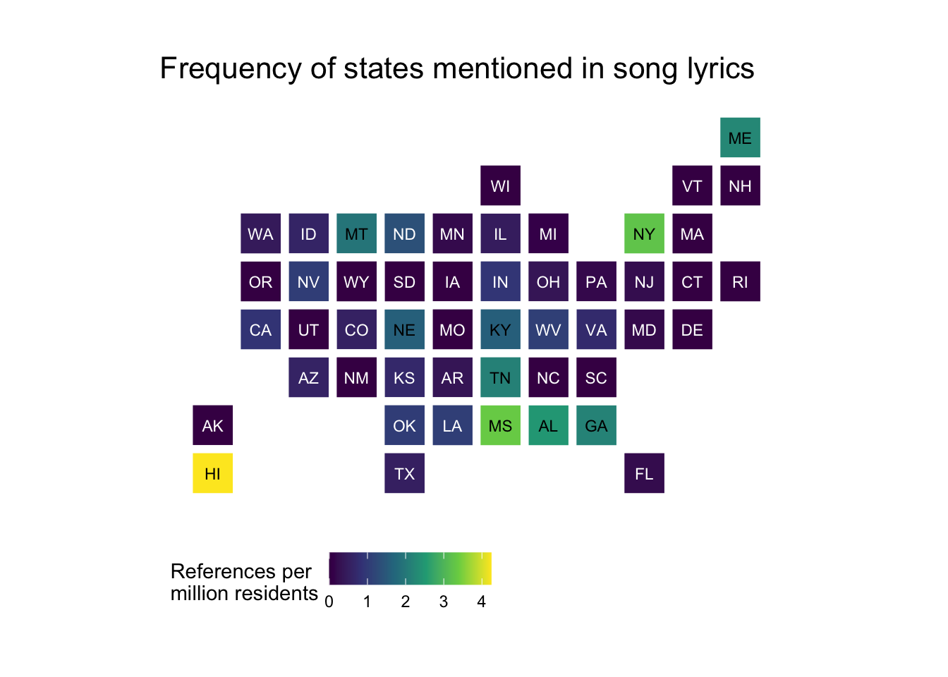
Now we can see that California and New York still referenced frequently, but but on a per-capita basis Hawaii is significantly overrepresented. The per capita rate of mentions for Hawaii is higher than for California or New York. This is because Hawaii is a small state with a small population, so even a few mentions in song lyrics can make a big difference in the per capita rate.
Acknowledgments
- This page is derived in part from SONG LYRICS ACROSS THE UNITED STATES and licensed under a Creative Commons Attribution-ShareAlike 4.0 International License.
Session information
sessioninfo::session_info()─ Session info ───────────────────────────────────────────────────────────────
setting value
version R version 4.3.1 (2023-06-16)
os macOS Ventura 13.5.2
system aarch64, darwin20
ui X11
language (EN)
collate en_US.UTF-8
ctype en_US.UTF-8
tz America/New_York
date 2024-01-05
pandoc 3.1.1 @ /Applications/RStudio.app/Contents/Resources/app/quarto/bin/tools/ (via rmarkdown)
─ Packages ───────────────────────────────────────────────────────────────────
package * version date (UTC) lib source
acs * 2.1.4 2019-02-19 [1] CRAN (R 4.3.0)
bit 4.0.5 2022-11-15 [1] CRAN (R 4.3.0)
bit64 4.0.5 2020-08-30 [1] CRAN (R 4.3.0)
class 7.3-22 2023-05-03 [1] CRAN (R 4.3.0)
classInt 0.4-10 2023-09-05 [1] CRAN (R 4.3.0)
cli 3.6.2 2023-12-11 [1] CRAN (R 4.3.1)
colorspace 2.1-0 2023-01-23 [1] CRAN (R 4.3.0)
crayon 1.5.2 2022-09-29 [1] CRAN (R 4.3.0)
curl 5.2.0 2023-12-08 [1] CRAN (R 4.3.1)
DBI 1.1.3 2022-06-18 [1] CRAN (R 4.3.0)
digest 0.6.33 2023-07-07 [1] CRAN (R 4.3.0)
dplyr * 1.1.4 2023-11-17 [1] CRAN (R 4.3.1)
e1071 1.7-14 2023-12-06 [1] CRAN (R 4.3.1)
evaluate 0.23 2023-11-01 [1] CRAN (R 4.3.1)
fansi 1.0.6 2023-12-08 [1] CRAN (R 4.3.1)
farver 2.1.1 2022-07-06 [1] CRAN (R 4.3.0)
fastmap 1.1.1 2023-02-24 [1] CRAN (R 4.3.0)
forcats * 1.0.0 2023-01-29 [1] CRAN (R 4.3.0)
generics 0.1.3 2022-07-05 [1] CRAN (R 4.3.0)
ggplot2 * 3.4.4 2023-10-12 [1] CRAN (R 4.3.1)
glue 1.6.2 2022-02-24 [1] CRAN (R 4.3.0)
gtable 0.3.4 2023-08-21 [1] CRAN (R 4.3.0)
here * 1.0.1 2020-12-13 [1] CRAN (R 4.3.0)
hms 1.1.3 2023-03-21 [1] CRAN (R 4.3.0)
htmltools 0.5.7 2023-11-03 [1] CRAN (R 4.3.1)
htmlwidgets 1.6.4 2023-12-06 [1] CRAN (R 4.3.1)
httr 1.4.7 2023-08-15 [1] CRAN (R 4.3.0)
janeaustenr 1.0.0 2022-08-26 [1] CRAN (R 4.3.0)
jsonlite 1.8.8 2023-12-04 [1] CRAN (R 4.3.1)
KernSmooth 2.23-22 2023-07-10 [1] CRAN (R 4.3.0)
knitr 1.45 2023-10-30 [1] CRAN (R 4.3.1)
labeling 0.4.3 2023-08-29 [1] CRAN (R 4.3.0)
lattice 0.22-5 2023-10-24 [1] CRAN (R 4.3.1)
lifecycle 1.0.4 2023-11-07 [1] CRAN (R 4.3.1)
lubridate * 1.9.3 2023-09-27 [1] CRAN (R 4.3.1)
magrittr 2.0.3 2022-03-30 [1] CRAN (R 4.3.0)
Matrix 1.6-4 2023-11-30 [1] CRAN (R 4.3.1)
munsell 0.5.0 2018-06-12 [1] CRAN (R 4.3.0)
pillar 1.9.0 2023-03-22 [1] CRAN (R 4.3.0)
pkgconfig 2.0.3 2019-09-22 [1] CRAN (R 4.3.0)
plyr 1.8.9 2023-10-02 [1] CRAN (R 4.3.1)
proxy 0.4-27 2022-06-09 [1] CRAN (R 4.3.0)
purrr * 1.0.2 2023-08-10 [1] CRAN (R 4.3.0)
R6 2.5.1 2021-08-19 [1] CRAN (R 4.3.0)
rappdirs 0.3.3 2021-01-31 [1] CRAN (R 4.3.0)
RColorBrewer 1.1-3 2022-04-03 [1] CRAN (R 4.3.0)
Rcpp 1.0.11 2023-07-06 [1] CRAN (R 4.3.0)
readr * 2.1.4 2023-02-10 [1] CRAN (R 4.3.0)
rlang 1.1.2 2023-11-04 [1] CRAN (R 4.3.1)
rmarkdown 2.25 2023-09-18 [1] CRAN (R 4.3.1)
rprojroot 2.0.4 2023-11-05 [1] CRAN (R 4.3.1)
rstudioapi 0.15.0 2023-07-07 [1] CRAN (R 4.3.0)
rvest 1.0.3 2022-08-19 [1] CRAN (R 4.3.0)
scales 1.3.0 2023-11-28 [1] CRAN (R 4.3.1)
sessioninfo 1.2.2 2021-12-06 [1] CRAN (R 4.3.0)
sf 1.0-14 2023-07-11 [1] CRAN (R 4.3.0)
SnowballC 0.7.1 2023-04-25 [1] CRAN (R 4.3.0)
statebins * 1.4.0 2020-07-08 [1] CRAN (R 4.3.0)
stringi 1.8.3 2023-12-11 [1] CRAN (R 4.3.1)
stringr * 1.5.1 2023-11-14 [1] CRAN (R 4.3.1)
tibble * 3.2.1 2023-03-20 [1] CRAN (R 4.3.0)
tidycensus * 1.5 2023-09-26 [1] CRAN (R 4.3.1)
tidyr * 1.3.0 2023-01-24 [1] CRAN (R 4.3.0)
tidyselect 1.2.0 2022-10-10 [1] CRAN (R 4.3.0)
tidytext * 0.4.1 2023-01-07 [1] CRAN (R 4.3.0)
tidyverse * 2.0.0 2023-02-22 [1] CRAN (R 4.3.0)
tigris 2.0.4 2023-09-22 [1] CRAN (R 4.3.1)
timechange 0.2.0 2023-01-11 [1] CRAN (R 4.3.0)
tokenizers 0.3.0 2022-12-22 [1] CRAN (R 4.3.0)
tzdb 0.4.0 2023-05-12 [1] CRAN (R 4.3.0)
units 0.8-5 2023-11-28 [1] CRAN (R 4.3.1)
utf8 1.2.4 2023-10-22 [1] CRAN (R 4.3.1)
uuid 1.1-1 2023-08-17 [1] CRAN (R 4.3.0)
vctrs 0.6.5 2023-12-01 [1] CRAN (R 4.3.1)
viridisLite 0.4.2 2023-05-02 [1] CRAN (R 4.3.0)
vroom 1.6.5 2023-12-05 [1] CRAN (R 4.3.1)
withr 2.5.2 2023-10-30 [1] CRAN (R 4.3.1)
xfun 0.41 2023-11-01 [1] CRAN (R 4.3.1)
XML * 3.99-0.16 2023-11-29 [1] CRAN (R 4.3.1)
xml2 1.3.6 2023-12-04 [1] CRAN (R 4.3.1)
yaml 2.3.8 2023-12-11 [1] CRAN (R 4.3.1)
[1] /Library/Frameworks/R.framework/Versions/4.3-arm64/Resources/library
──────────────────────────────────────────────────────────────────────────────